‘Parking Downhill’ & Spatial Data Fundamentals

Overview

Under Construction

Learning Objectives

TBD

Preparation

TBD

Park Downhill

Beyond preserving and promoting the current work, there are a few things you can do to prepare for the new research opportunities that it can generate. Ideally, the group has been tracking spin-off ideas as they come up. It’s impractical to chase them all down in the moment, but recording them, with just a few sentences of context and explanation, will help to resurface the inspiration at a later date.

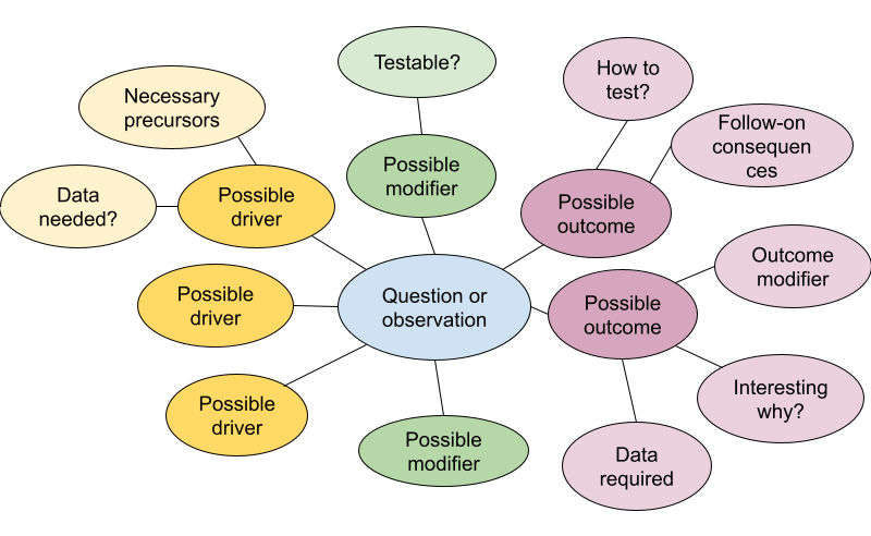
Now is the time to pull those ideas out of mothballs or, alternatively, return to the mind maps we made in the project management session to unearth some new ones.

This year, you’ve tackled one, maybe two, of the relationships on that mind map. But chances are that the data you’ve assembled sheds light on several more. In this project group discussion, we’ll take some time to identify and explore a few of them.

Discussion: Preparing to Propose

Part 1 - Individually

Pull up your running list of project ideas, the mind map you generated in the project management session, or start a new mind map with your current project theme at the center.
Come up with a related research idea that capitalizes on the data you’ve assembled. Try focusing on upstream controls, downstream impacts or modifying factors to spur your creativity. It doesn’t have to be Nobel-worthy, it’s just for this exercise.
Identify what additional data or analyses would be needed to clarify the nature and scale of the relationship
How might a change in our understanding of that relationship affect how we understand other processes?

Part 2 - In Pairs

Explain your idea, what you would need, and where it might lead

Part 3 - Still in Pairs

For each of your projects, brainstorm a list of people (individuals, groups, roles, agencies) who care about those changes or that might benefit from or be hurt by them.
For example, say your original project was focused on understanding what factors influence the long term immobilization of soil carbon during decomposition. Spin-off ideas might look at:
- Additional controlling factors that you couldn’t include in the first effort;
- A wider range of ecosystems;
- The role of variability (not only temperature, for example, but also the frequency of freeze-thaw cycles);
- The effect of the same factors on the mobilization of nutrients in soil; or
- Scaling the analysis to forecast the impact on carbon sinks under alternative climate scenarios.
In addition to the standard science funding agencies such as NSF, NASA, DOE, or USDA, other interested parties: farmers, fertilizer suppliers, extension professionals, carbon markets, climate modelers…
- Note these along with the nature of their interest.

Part 4 - In Full Group

Discuss how ideas came together and what kinds of audiences were identified.

a garment pocket with money poking out of it

When thinking about how to support a research program, strategy (setting goals and making plans to achieve them) is often contrasted with an opportunistic approach. But really, it’s essential to apply a bit of both. The list of people and agencies you generated from this exercise serves as a starting point for exploring funding opportunities. When you find an opportunity that intersects with a problem that you have the tools, skills, and data to tackle, that’s when you spring into action, building on knowledge gaps that you’ve already identified.

When you have an idea that you’re excited about, one great practice is to develop a “pocket proposal”–a two-page, scaled down description of the research you hope to do. Writing one will force you to clarify your ideas, improve your articulation of them, give you something to share with colleagues (either to invite collaborators or to seek critical feedback), and provide a head start when you DO find a funding opportunity that’s a fit.

Bonus!

A pocket proposal serves as a great starting point for the research statement you’ll need for a faculty job search.

Crafting a Compelling Proposal

No matter your audience, you need to put yourself in their shoes. Decision makers spend their limited resources to meet their goals, no matter how exciting they find your science. Of course you need to follow their guidelines, but take it a step further. Think about who this agency serves. Read up on their past awards. Get inside their heads.

Pro-tip

All NSF program pages have a link at the bottom leading to a list of past awards made through the program. Successful proposers are often quite happy to share their funded proposal.

The bones of any proposal include answers to the following questions:

Context - what is already known/done? What’s the gap you’re trying to fill?
What do you want to do?
How do you plan to do it?
Why are you the right person/group to do it?
Why is it a fit for THIS funder?
How will you disseminate or apply the work?
What do you expect the results to be

Depending on the source of funding, the order and emphasis of these items will be different. For a foundation funder, the need and results might be most important, with the precise “how” taking a back seat. For a science agency, context and work plan will take higher priority, but be sure to include why you are the right group to do it and what you expect the results to be–even if only a sentence or two.

Even for an individual donor, you’ll want to have a list of talking points that addresses these questions, but you probably won’t turn it into a formal proposal until you’ve developed a relationship.

It can be intimidating, but it is immensely helpful to ask for feedback from experienced colleagues at various stages of proposal development. Be sure to specify what kind of feedback would be useful to you and to give them a (reasonable) deadline.

Discussion: Revisit Group Authorship Agreement

With a partner/group discuss (some of) the following questions:

Anytime a project undergoes a major transition, it’s a good idea to revisit the approach to authorship. An agreement that worked well for an organized project with fixed membership may not be as appropriate for spin-off projects, spearheaded by individual team members and involving rotating groups of collaborators.

Break out into project groups and discuss the following questions as they might apply to emerging projects:

Do we know of any emerging projects?
Who wants to stay involved? In what ways?
When related research opportunities arise, is there a responsibility to notify the group? To invite participation?
Whether a team member wants to stay involved or not, what are the expectations for how members of this group are credited on future related projects?

Record the decisions and preserve for further discussion as projects evolve.

Needed Packages

If you’d like to follow along with the code chunks included throughout this module, you’ll need to install the following packages:

# Note that these lines only need to be run once per computer
## So you can skip this step if you've installed these before
install.packages("tidyverse")
install.packages("sf")
install.packages("terra")
install.packages("maps")
install.packages("exactextractr")

Types of Spatial Data

There are two main types of spatial data: vector and raster. Both types (and the packages they require) are described in the tabs below.

Vector data are stored as polygons. Essentially vector data are a set of points and–sometimes–the lines between them that define the edges of a shape. They may store additional data that is retained in a semi-tabular format that relates to the polygon(s) but isn’t directly stored in them.

Common vector data types include shape files or GeoJSONs.

# Load needed library
library(sf)

# Read in shapefile
nc_poly <- sf::st_read(dsn = file.path("data", "nc_borders.shp"))

1: Note that even though we’re only specifying the “.shp” file in this function you must also have the associated files in that same folder. In this case that includes a “.dbf”, “.prj”, and “.shx”, though in other contexts you may have others.

Once you have read in the shapefile, you can check its structure as you would any other data object. Note that the object has both the ‘data.frame’ class and the ‘sf’ (“simple features”) class. In this case, the shapefile relates to counties in North Carolina and some associated demographic data in those counties.

# Check structure
str(nc_poly)

Classes 'sf' and 'data.frame':  100 obs. of  15 variables:
 $ AREA     : num  0.114 0.061 0.143 0.07 0.153 0.097 0.062 0.091 0.118 0.124 ...
 $ PERIMETER: num  1.44 1.23 1.63 2.97 2.21 ...
 $ CNTY_    : num  1825 1827 1828 1831 1832 ...
 $ CNTY_ID  : num  1825 1827 1828 1831 1832 ...
 $ NAME     : chr  "Ashe" "Alleghany" "Surry" "Currituck" ...
 $ FIPS     : chr  "37009" "37005" "37171" "37053" ...
 $ FIPSNO   : num  37009 37005 37171 37053 37131 ...
 $ CRESS_ID : int  5 3 86 27 66 46 15 37 93 85 ...
 $ BIR74    : num  1091 487 3188 508 1421 ...
 $ SID74    : num  1 0 5 1 9 7 0 0 4 1 ...
 $ NWBIR74  : num  10 10 208 123 1066 ...
 $ BIR79    : num  1364 542 3616 830 1606 ...
 $ SID79    : num  0 3 6 2 3 5 2 2 2 5 ...
 $ NWBIR79  : num  19 12 260 145 1197 ...
 $ geometry :sfc_MULTIPOLYGON of length 100; first list element: List of 1
  ..$ :List of 1
  .. ..$ : num [1:27, 1:2] -81.5 -81.5 -81.6 -81.6 -81.7 ...
  ..- attr(*, "class")= chr [1:3] "XY" "MULTIPOLYGON" "sfg"
 - attr(*, "sf_column")= chr "geometry"
 - attr(*, "agr")= Factor w/ 3 levels "constant","aggregate",..: NA NA NA NA NA NA NA NA NA NA ...
  ..- attr(*, "names")= chr [1:14] "AREA" "PERIMETER" "CNTY_" "CNTY_ID" ...

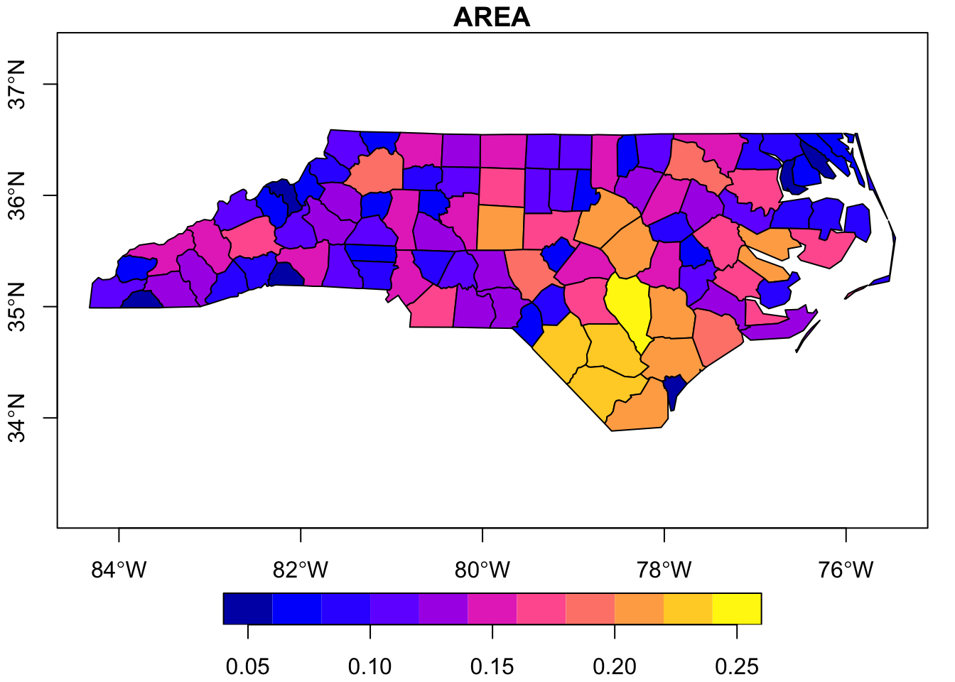
If desired, we could make a simple R base plot-style map. In this case we’ll do it based on just the county areas so that the polygons are filled with a color corresponding to how large the county is.

# Make a graph
plot(nc_poly["AREA"], axes = T)

Raster data are stored as values in pixels. The resolution (i.e., size of the pixels) may differ among rasters but in all cases the data are stored at a per-pixel level.

Common raster data types include GeoTIFFs (.tif) and NetCDF (.nc) files.

# Load needed library
library(terra)

# Read in raster
nc_pixel <- terra::rast(x = file.path("data", "nc_elevation.tif"))

Once you’ve read in the raster file you can check it’s structure as you would any other object but the resulting output is much less informative than for other object classes.

# Check structure
str(nc_pixel)

S4 class 'SpatRaster' [package "terra"]

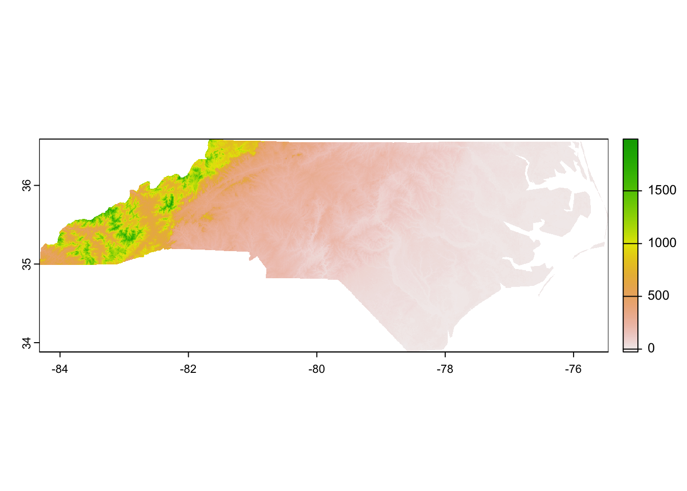
Regardless, now that we have the raster loaded we can make a simple graph to check out what sort of data is stored in it. In this case, each pixel is 3 arcseconds on each side (~0.0002° latitude/longitude) and contains the elevation (in meters) of that pixel.

# Make a graph
terra::plot(nc_pixel)

Coordinate Reference Systems

A fundamental problem in spatial data is how to project data collected on a nearly spherical planet onto a two-dimensional plane. This has been solved–or at least clarified–by the use of Coordinate Reference Systems (a.k.a. “CRS”). All spatial data have a CRS that is explicitly identified in the data and/or the metadata because the data are not interpretable without knowing which CRS is used.

The CRS defines the following information:

Datum – model for shape of the Earth including the starting coordinate pair and angular units that together define any particular point on the planet
- Note that there can be global datums that work for any region of the world and local datums that only work for a particular area
Projection – math for the transformation to get from a round planet to a flat map
Additional parameters – any other information necessary to support the projection
- E.g., the coordinates at the center of the map

Some people use the analogy of peeling a citrus fruit and flattening the peel to describe the components of a CRS. The datum is the choice between a lemon or a grapefruit (i.e., the shape of the not-quite-spherical object) while the projection is the instructions for taking the complete peel and flattening it.

You can check and transform the CRS in any scripted language that allows the loading of spatial data though the specifics do differ between the types of spatial data we introduced earlier.

For vector data we can check the CRS with other functions from the sf library. It can be a little difficult to parse all of the information that returns but essentially it is most important that the CRS match that of any other spatial data with which we are working.

# Check CRS
sf::st_crs(x = nc_poly)

Once you know the CRS, you can transform the data to another CRS if desired. This is a relatively fast operation for vector data because we’re transforming geometric data rather than potentially millions of pixels.

# Transform CRS
nc_poly_nad83 <- sf::st_transform(x = nc_poly, crs = 3083)

# Re-check CRS
sf::st_crs(nc_poly_nad83)

1: In order to transform to a new CRS you’ll need to identify the four-digit EPSG code for the desired CRS.

For raster data we can check the CRS with other functions from the terra library. It can be a little difficult to parse all of the information that returns but essentially it is most important that the CRS match that of any other spatial data with which we are working.

# Check CRS
terra::crs(nc_pixel)

As with vector data, if desired you can transform the data to another CRS. However, unlike vector data, transforming the CRS of raster data is very computationally intense. If at all possible you should avoid re-projecting rasters. If you must re-project, consider doing so in an environment with greater computing power than a typical laptop. Also, you should export a new raster in your preferred CRS after transforming so that you reduce the likelihood that you need to re-project again later in the lifecylce of your project.

In the interests of making this website reasonably quick to re-build, the following code chunk is not actually evaluated but is the correct syntax for this operation.

# Transform CRS
nc_pixel_nad83 <- terra::project(x = nc_pixel, y = "epsg:3083")

# Re-check CRS
terra::crs(nc_pixel_nad83)

Making Maps

Now that we’ve covered the main types of spatial data as well as how to check the CRS (and transform if needed) we’re ready to make maps! For consistency with other modules on data visualization, we’ll use ggplot2 to make our maps but note that base R also supports map making and there are many useful tutorials elsewhere on making maps in that framework.

The maps package includes some useful national and US state borders so we’ll begin by preparing an object that combines both sets of borders.

# Load library
library(maps)

# Make 'borders' object
borders <- sf::st_as_sf(maps::map(database = "world", plot = F, fill = T)) %>%
  dplyr::bind_rows(sf::st_as_sf(maps::map(database = "state", plot = F, fill = T)))

Note that the simplest way of making a map that includes a raster is to coerce that raster into a dataframe. To do this we will translate each pixel’s geographic coordinates into X and Y values.

nc_pixel_df <- as.data.frame(nc_pixel, xy = T) %>% 
    # Rename the 'actual' data layer more clearly
    dplyr::rename(elevation_m = SRTMGL3_NC.003_SRTMGL3_DEM_doy2000042_aid0001)

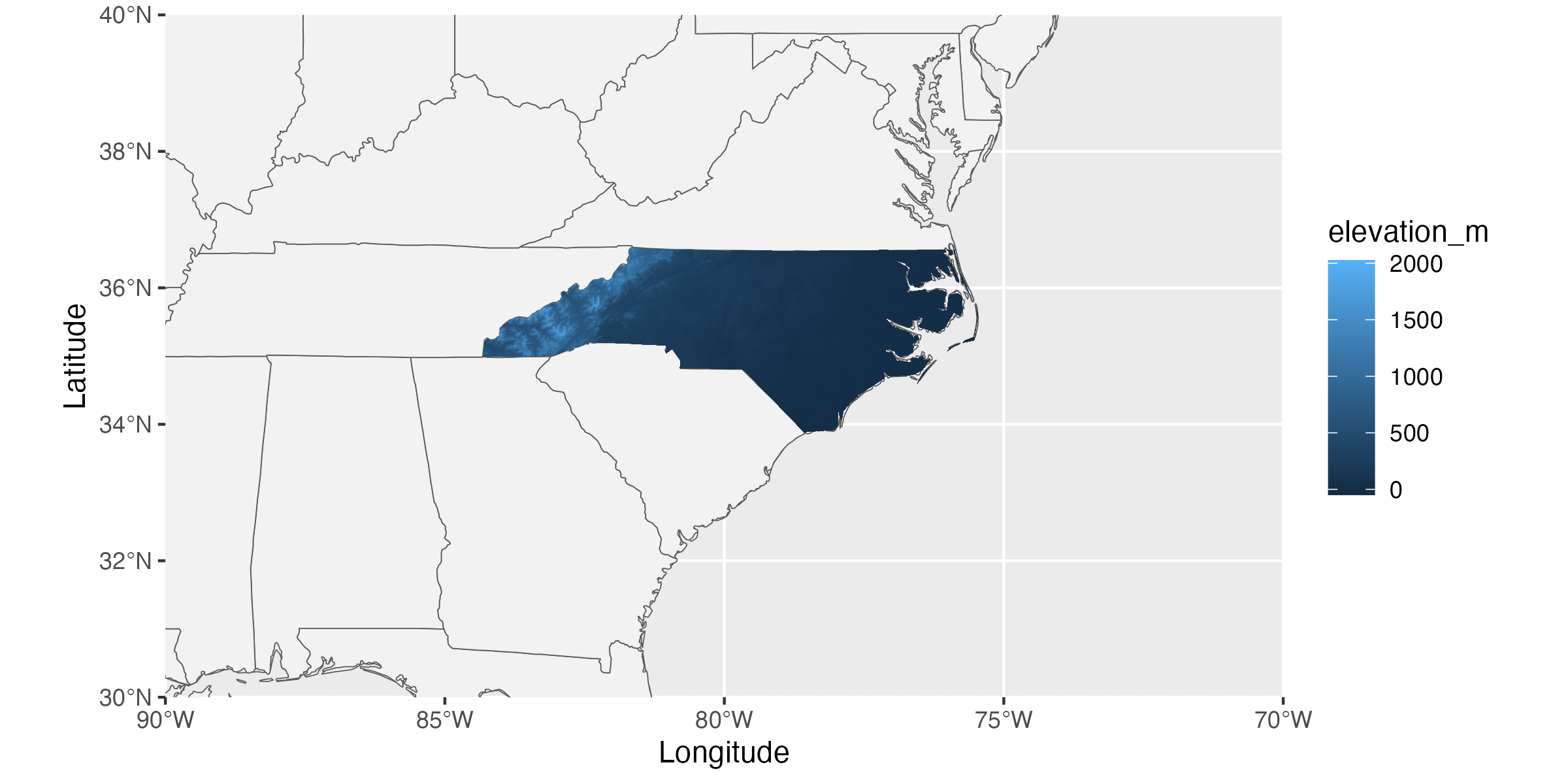
With the borders object and our modified raster in hand, we can now make a map that includes useful context for state/nation borders. Synthesis projects often cover a larger geographic extent than primary projects so this is particularly useful in ways it might not be for primary research.

# Load library
library(ggplot2)

# Make map
ggplot(borders) +
  geom_sf(fill = "gray95") +
  coord_sf(xlim = c(-70, -90), ylim = c(30, 40), expand = F) +
  geom_tile(data = nc_pixel_df, aes(x = x, y = y, fill = elevation_m)) +
  labs(x = "Longitude", y = "Latitude")

1: This line is filling our nation polygons with a pale gray (helps to differentiate from ocean)
2: Here we set the map extent so that we’re only getting our region of interest

ggplot2-style map of the southeastern US where North Carolina is colored based on the per-pixel elevation

From here we can make additional ggplot2-style modifications as/if needed. This variant of map-making supports adding tabular data objects as well (though they would require separate geometries). Many of the LTER Network Office-funded groups that make maps include points for specific study locations along with a raster layer for an environmental / land cover characteristic that is particularly relevant to their research question and/or hypotheses.

Extracting Spatial Data

By far the most common spatial operation that LNO-funded synthesis working groups want to perform is extraction of some spatial covariate data within their region of interest. “Extraction” here includes (1) the actual gathering of values from the desired area, (2) summarization of those values, and (3) attaching those summarized values to an existing tabular dataset for further analysis/visualization. As with any coding task there are many ways of accomplishing this end but we’ll focus on one method in the following code chunks: extraction in R via the exactextractr package.

This package expects that you’ll want to extract raster data within a the borders described in some type of vector data. If you want the values in all the pixels of a GeoTIFF that fall inside the boundary defined by a shapefile, tools in this package will be helpful.

We’ll begin by making a simpler version of our North Carolina vector data. This ensures that the extraction is as fast as possible for demonstrative purposes while still being replicable for you.

# Simplify the vector data
nc_poly_simp <- nc_poly %>% 
  dplyr::filter(NAME %in% c("Wake", "Swain")) %>% 
  dplyr::select(NAME, AREA)

# Check structure to demonstrate simplicity
dplyr::glimpse(nc_poly_simp)

1: Note that even though we used select to remove all but one column, the geometry information is retained!

Now let’s use this simplified object and extract elevation for our counties of interest (normally we’d likely do this for all counties but the process is the same).

# Load needed libraries
library(exactextractr)
library(purrr)

# Perform extraction
extracted_df <- exactextractr::exact_extract(x = nc_pixel, y = nc_poly_simp,
                                             include_cols = c("NAME", "AREA"),
                                             progress = F) %>%
  # Collapse to a dataframe
  purrr::list_rbind(x = .)

# Check structure
dplyr::glimpse(extracted_df)

1: Note that functions like this one assume that both spatial data objects use the same CRS. We checked that earlier so we’re good but remember to include that check every time you do something like this!
2: All column names specified here from the vector data (see the y argument) will be retained in the output. Otherwise only the extracted value and coverage fraction are included.
3: This argument controls whether a progress bar is included. Extremely useful when you have many polygons / the extraction takes a long time!
4: The default output of this function is a list with one dataframe of extracted values per polygon in your vector data so we’ll unlist to a dataframe for ease of future operations

In the above output we can see that it has extracted the elevation of every pixel within each of our counties of interest and provided us with the percentage of that pixel that is covered by the polygon (i.e., by the shapefile). We can now summarize this however we’d like and–eventually–join it back onto the county data via the column(s) we specified should be retained from the original vector data.