# Load the supportR package
library(supportR)Building Consensus & Checking the Data
This module is focused on how your group might build consensus, particularly with regard to specific hypotheses or research questions that fit within your larger project frame. We’ll also discuss some checks you may want to run on your data and specific functions in R that perform those operations.
Collaborative Convergence
At the beginning of a collaborative process, the most important initial outcome is getting convergence or group alignment on a set of shared goals and objectives and a plan for how to achieve them. If your team process is effective, this plan will be an inclusive solution–one that works for everyone in the group. Achieving this shared vision can be more difficult than one might expect. While you may expect that participants have already agreed to the vision in joining the group, agreement does not always equate to alignment. This module focuses on tools and resources to help your group navigate to convergent, inclusive solutions that everyone on the team can align around.
Embracing Divergent Thinking
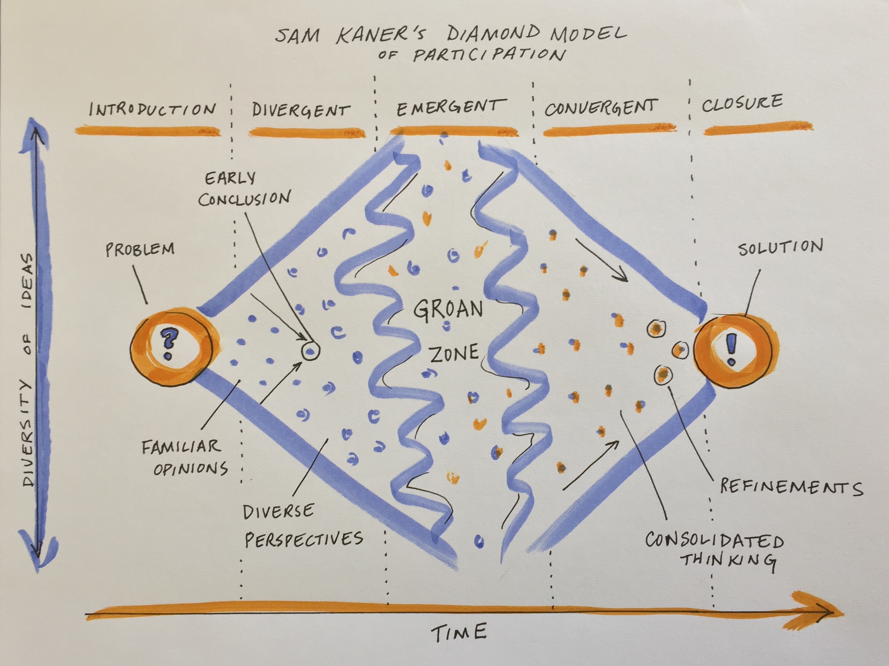
The first stage of group decision making is divergent thinking (Kaner et al. 2014). Confronted with a new, complex topic, the group will gradually move from the safe territory of familiar opinions into sharing their diverse perspectives and exploring new ideas. This can feel like the group process is devolving away from what was assumed to be shared agreement, but it is actually a critical part of the collaborative process.
When a diverse group comes together to work on a complex problem, their views are likely to diverge widely across many dimensions from problem definition to priorities to methods/approaches to the definition of success. But you can tap that divergent thinking to generate entirely new ideas and options that emerge through the group’s productive struggle for mutual understanding.
While your working group is in the divergent thinking stage, it’s critical to foster dialogue to surface different perspectives. Examine hidden assumptions. Create room for disagreement and questioning. Amplify diverse perspectives–and particularly, voices from the edge (e.g., junior members, new collaborators, people from different disciplines, non-scientists who may be affected by the research)–in order to expand the range of possibilities. Mirror and validate what you hear. Invite people who are good at bridging across disciplinary or other differences to help translate and build shared understanding of methods and ways of thinking. Suspend judgment and encourage full participation.
Beware of the most common pitfall at this stage, which is to converge too quickly on an early conclusion, staying in the safe space of familiar opinions and status quo solutions. You can prepare for this stage and help to avoid that pitfall by reviewing prior work and synthesizing data and knowledge gaps, promising approaches, and critical questions. Your team can use that synthesis of the current state of the science as a jumping off point.
Making it Through the Groan Zone
It’s natural for groups to go through a period of confusion and frustration as they struggle to integrate their diverse perspectives into a shared framework of understanding (Kaner et al. 2014). The goal is to get the group across this no man’s land between divergent thinking and convergence known as the “groan zone”. In the groan zone, the group leader or facilitator’s job is to keep the group from getting frustrated and shutting down.
While the groan zone can be challenging, it can also be an extremely fruitful and creative stage. Here in the messy middle of a group process, an open and flexible mindset and a process that invites participants to engage in emergent thinking can enable true innovation. Emergent thinking builds upon ideas generated in the divergent thinking stage, recombining or adapting them in novel ways. It seeks to identify patterns and make meaning in the face of complexity and uncertainty. Done well, emergent thinking enables a group to adapt, sense opportunities, and generate new and exciting ideas.
Some useful techniques for navigating the groan zone and fostering emergent thinking include:
- Cultivating presence and patience
- Active listening
- Building shared understanding via translation (e.g. across disciplines), metacognition (thinking about how you are thinking), and inquiry
- Exploring new data, models, and ways of presenting information
- Creating categories to reveal structure and allow sorting and prioritization of ideas
- Combining or recombining ideas or methods to yield new approaches
- Working together to separate facts from opinions
- Carefully examining language, e.g. by looking word by word at a key statement or question that is being debated and asking what questions each word raises
- Capturing side issues in writing and reserving time to revisit these – taking the tangents seriously is a critical part of letting participants know you value their contributions
- Examining how proposed ideas might affect each individual in the group
- Honoring objections to the process and asking for suggestions
- Addressing power imbalances and elevating voices from the “edge”
Some typical obstacles to emergent thinking include:
- Disciplinary differences in epistemology, vocabulary, and methods that impede understanding
- Analysis paralysis - getting lost in the weeds of endless analysis and detail
- Polarization - opposite camps anchored in
- Power dynamics that squelch creative contributions from the “edges”
- Avoidance of a deeper issue impeding collaboration (e.g. lack of trust)
- Turf wars, competition
- Risk aversion, perception management, fear of failure / getting it wrong
- Confirmation bias and resistance to ideas that challenge group identity and beliefs
If you find the conversation getting off track or the dynamics becoming difficult, useful techniques that allow you to remain committed to being supportive and respectful of all group members (including ones you might experience as “difficult”) include:
- Reminding individuals of the larger purpose of the group and reconnecting them to their own personal reasons for caring about and working on the issue, e.g. by inviting them to take a moment to reflect or to restate what success looks like
- Focusing on common ground and areas of potential alignment
- Inviting constructive opposition - ask the critic to say what they can support about a given proposal and what they would like to see changed or discussed further
- Switching the participation format (e.g., going to breakout groups, brainstorming, a go-around, or individual writing)
- Taking a break
- Stepping out of the content and addressing the process
- Educating members about group dynamics and asking them to reflect on how they are showing up
- Encouraging more people to participate
- Reframing the discussion, e.g. by surfacing underlying issues, and/or focusing on concrete actions that the group can take to resolve the conflict
Don’t get discouraged by the groan zone. Misunderstanding and miscommunication are normal parts of the process of collaboration. And even more importantly, “the act of working through these misunderstandings is what builds the foundation for sustainable agreements [and]… meaningful collaboration” (Kaner et al. 2014).
Getting to Convergence
Once the group has a strong foundation of shared understanding, things often start to click into place and feel easier and faster as you enter the zone of convergent thinking. At this point, the group is ready to devise inclusive solutions, weigh alternatives and make decisions. As the group leader your role is to help the group devise specific proposals, evaluate and decide among them, refine and synthesize into an overall approach, and lay out a concrete plan. The risk at this stage is that the group never converges on a clear decision or plan, leading the group to spin its wheels in the future.
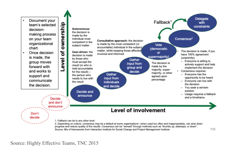
Discuss as a team how you want to make decisions - what is your decision making process going to be? Will it be based on consensus? Majority rules? Or will you delegate the decisionmaking to the team leader or a sub-team who are closest to the decision? What’s your fallback plan if you can’t reach a decision during your time together? The figure below arrays a variety of different decisionmaking processes onto the axes of level of group member involvement and level of group member ownership. Note that the two red circles that are off the graph in the bottom left should definitely be avoided!
Techniques that are useful in this phase include:
- Pulling up concrete examples for inspiration
- Inviting concrete, written proposals
- Clarifying selection criteria and evaluating proposals against them
- Combining the best elements of multiple ideas to support more innovative, inclusive solutions
- Deciding what ideas to pursue and which to keep on the back burner in case the team needs to adapt
- Defining steps and milestones, planning the work flow, and assigning roles and responsibilities
While the big work of the initial stage of a synthesis science project is getting to convergence on the overall work plan, you should expect that the group may go through the process of divergence and convergence again at multiple points in the process as you dive into the work and uncover new challenges. But the shared understanding and social rapport that come from successfully struggling together early on will allow the group to more easily and rapidly develop and implement new solutions in subsequent meetings.
Quality Control
You may have encountered the phrase “QA/QC” (Quality Assurance / Quality Control) in relation to data cleaning. Technically, quality assurance only encapsulates preventative measures for reducing errors. One example of QA would be using a template for field datasheets because using standard fields reduces the risk that data are recorded inconsistently and/or incompletely. Quality control on the other hand refers to all steps taken to resolve errors after data are collected. Any code that you write to fix typos or remove outliers from a dataset falls under the umbrella of QC.
In synthesis work, QA is only very rarely an option. You’ll mostly be working with datasets that have already been collected and attempting to handle any issues post hoc which means the vast majority of data wrangling operations will be quality control methods. These QC efforts can be incredibly time-consuming so using a programming language (like R or Python) is a dramatic improvement over manually looking through the data using Microsoft Excel or other programs like it.
QC Considerations
The datasets you gather for your synthesis project will likely have a multitude of issues you’ll need to resolve before the data are ready for visualization or analysis. Some of these issues may be clearly identified in that datasets’ metadata or apply to all datasets but it is good practice to make a thorough QC effort as early as is feasible. Keep the following data issues and/or checks in mind as we cover code tools that may be useful in this context later in the module.
- Verify taxonomic classifications against authorities
- Handle missing data
- Some datasets will use a code to indicate missing values (likely identified in their metadata) while others will just have empty cells
- Check for unreasonable values / outliers
- Can use conditionals to create “flags” for these values or just filter them out
- Check geographic coordinates’ reasonability
- E.g., western hemisphere coordinates may lack the minus sign
- Check date formatting
- I.e., if all sampling is done in the first week of each month it can be difficult to say whether a given date is formatted as MM/DD/YY or DD/MM/YY
- Consider spatial and temporal granularity among datasets
- You may need to aggregate data from separate studies in different ways to ensure that the data are directly comparable across all of the data you gather
- Handle duplicate data / rows
Number Checking
When you read in a dataset and a column that should be numeric is instead read in as a character, it can be a sign that there are malformed numbers lurking in the background. Checking for and resolving these non-numbers is preferable to simply coercing the column into being numeric because the latter method typically changes those values to ‘NA’ where a human might be able to deduce the true number each value ‘should be.’
# Create an example dataset with non-numbers in ideally numeric columns
fish_ct <- data.frame("species" = c("salmon", "bass", "halibut", "moray eel"),
                      "count" = c(12, "14x", "_23", 1))

# Check for malformed numbers in column(s) that should be numeric
bad_nums <- supportR::num_check(data = fish_ct, col = "count")
For 'count', 2 non-numbers identified: '14x' | '_23'In the above example, “14x” would be coerced to NA if you simply force the column without checking but you could drop the “x” with text replacing methods once you use tools like this one to flag it for your attention.
Text Replacement
One of the simpler ways of handling text issues is just to replace a string with another string. Most programming languages support this functionality.
# Use pattern match/replace to simplify problem entries
fish_ct$count <- gsub(pattern = "x|_", replacement = "", x = fish_ct$count)

# Check that they are fixed
bad_nums <- supportR::num_check(data = fish_ct, col = "count")
For 'count', no non-numeric values identified.The vertical line in the gsub example above lets us search for (and replace) multiple patterns. Note however that while you can search for many patterns at once, only a single replacement value can be provided with this function.
Regular Expressions
You may sometimes want to perform more generic string matching where you don’t necessarily know–or want to list–all possible strings to find and replace. For instance, you may want remove any letter in a numeric column or find and replace numbers with some sort of text note. “Regular expressions” are how programmers specify these generic matches and using them can be a nice way of streamlining code.
# Make a test vector
regex_vec <- c("hello", "123", "goodbye", "456")

# Find all numbers and replace with the letter X
gsub(pattern = "[[:digit:]]", replacement = "x", x = regex_vec)
[1] "hello" "xxx" "goodbye" "xxx" # Replace any number of letters with only a single 0
gsub(pattern = "[[:alpha:]]+", replacement = "0", x = regex_vec)[1] "0" "123" "0" "456"The stringr package cheatsheet has a really nice list of regular expression options that you may find valuable if you want to delve deeper on this topic. Scroll to the second page of the PDF to see the most relevant parts.
Custom Functions
Writing your own functions can be really useful, particularly when doing synthesis work. Custom functions are generally useful for reducing duplication and increasing ease of maintenance. They may also become end products of synthesis work in and of themselves!
If one of your group’s outputs is a new standard data format or analytical workflow, the functions that you develop to aid yourself become valuable to anyone who adopts your synthesis project’s findings into their own workflows. If you get enough functions you can even release a package that others can install and use on their own computers. Such packages are a valuable product of synthesis efforts and can be a nice addition to a robust scientific resume or CV.
Core Function Writing Process
There are a number of ways one might go about writing a function, this topic will focus on one that is fairly flexible and should be applicable to most contexts you’re likely to run into in a synthesis context.
To make this more tangible, let’s load a dataset from the lterdatasampler package. We’ll use a dataset collected at the Niwot Ridge LTER on American Pika (Ochotona princeps) stress and habitat. You can see the full metadata for this dataset on the Environmental Data Initiative’s (EDI) website (Package ID: knb-lter-nwt.268.1).
# Load the needed libraries (install if needed)
## install.packages("librarian")
librarian::shelf(lterdatasampler, dplyr)
# Load the dataset and assign to an object
pika_df <- lterdatasampler::nwt_pikas
# Check the structure
str(pika_df)- 1
- Just doing this to have a shorter object name to refer to as we continue
tibble [109 × 8] (S3: tbl_df/tbl/data.frame)
 $ date              : Date[1:109], format: "2018-06-08" "2018-06-08" ...
 $ site              : Factor w/ 3 levels "Cable Gate","Long Lake",..: 1 1 1 3 3 3 3 3 3 3 ...
 $ station           : Factor w/ 20 levels "Cable Gate 1",..: 1 2 3 14 15 16 17 18 19 9 ...
 $ utm_easting       : num [1:109] 451373 451411 451462 449317 449342 ...
 $ utm_northing      : num [1:109] 4432963 4432985 4432991 4434093 4434141 ...
 $ sex               : Factor w/ 1 level "male": 1 1 1 1 1 NA 1 NA 1 1 ...
 $ concentration_pg_g: num [1:109] 11563 10629 10924 10414 13531 ...
$ elev_m : num [1:109] 3343 3353 3358 3578 3584 ...The first step of writing your own function is something you’d likely already do: write normal, non-function code that does what you want!
In this case, let’s say we’re interested in extracting the results of a simple linear model into a tidy table. This is a classic context for a custom function because we’ll fit many models and likely will want to just copy/paste those results into our manuscript.
# Fit one linear model
pika_mod <- lm(concentration_pg_g ~ site, data = pika_df)
# Get the summary of the model and assign that to an object
pika_result <- summary(pika_mod)
# Extract the coefficient table as a dataframe
pika_coef <- as.data.frame(pika_result$coefficients)
# The terms are preserved as row names but we'll need them as columns
pika_coef2 <- pika_coef |>
dplyr::mutate(terms = rownames(pika_coef),
.before = dplyr::everything()) |>
# Rename columns to avoid spaces and special characters
dplyr::rename(estimate = Estimate,
std.error = `Std. Error`,
t.value = `t value`,
p.value = `Pr(>|t|)`) |>
# Grab theadjusted R2 as well
dplyr::mutate(adj.r.squared = pika_result$adj.r.squared)
# Finally, ditch the superseded row names
rownames(pika_coef2) <- NULL
# Does that look like what we want?
pika_coef2- 1
- Here, we are testing whether the concentration of a stress-related metabolite differs among sites
- 2
-
We’re using R’s “native pipe” (
|>) to avoidmagrittras a “dependency” (i.e., a package required by our function) - 3
- Namespace ALL functions when you’re planning on writing a function so that there’s no chance that the order in which a user loads their packages breaks your function. It’s okay to skip base R function namespacing for brevity’s sake
- 4
- Note the adjusted R2 is found in a different part of the result object (rather than the coefficient object where the rest of the results table can be found)
           terms  estimate std.error    t.value      p.value adj.r.squared
1    (Intercept) 5412.2965  670.5996  8.0708315 1.162802e-12   -0.01576036
2  siteLong Lake -682.7670 1203.7631 -0.5671938 5.717817e-01   -0.01576036
3 siteWest Knoll -244.9262  749.7532 -0.3266758 7.445572e-01   -0.01576036
Step 1: Nitty Gritty
In order to write something like the above, you’ll (likely) need to do some experimenting to figure out where in each data object the information you want lives! This might look something like the following.
# Fit one linear model
pika_mod <- lm(concentration_pg_g ~ site, data = pika_df)
# Get the summary of the model and assign that to an object
pika_result <- summary(pika_mod)
# Check the structure of the 'results' object
str(pika_result)- 1
-
Here we can see the “coefficients” element has what we want but in some cases you may need to manually check each element (i.e., by running
str) until you find the one(s) that have what you want
List of 11
 $ call         : language lm(formula = concentration_pg_g ~ site, data = pika_df)
 $ terms        :Classes 'terms', 'formula'  language concentration_pg_g ~ site
  .. ..- attr(*, "variables")= language list(concentration_pg_g, site)
  .. ..- attr(*, "factors")= int [1:2, 1] 0 1
  .. .. ..- attr(*, "dimnames")=List of 2
  .. .. .. ..$ : chr [1:2] "concentration_pg_g" "site"
  .. .. .. ..$ : chr "site"
  .. ..- attr(*, "term.labels")= chr "site"
  .. ..- attr(*, "order")= int 1
  .. ..- attr(*, "intercept")= int 1
  .. ..- attr(*, "response")= int 1
  .. ..- attr(*, ".Environment")=<environment: R_GlobalEnv>
  .. ..- attr(*, "predvars")= language list(concentration_pg_g, site)
  .. ..- attr(*, "dataClasses")= Named chr [1:2] "numeric" "factor"
  .. .. ..- attr(*, "names")= chr [1:2] "concentration_pg_g" "site"
 $ residuals    : Named num [1:109] 6151 5217 5511 5246 8363 ...
  ..- attr(*, "names")= chr [1:109] "1" "2" "3" "4" ...
 $ coefficients : num [1:3, 1:4] 5412 -683 -245 671 1204 ...
  ..- attr(*, "dimnames")=List of 2
  .. ..$ : chr [1:3] "(Intercept)" "siteLong Lake" "siteWest Knoll"
  .. ..$ : chr [1:4] "Estimate" "Std. Error" "t value" "Pr(>|t|)"
 $ aliased      : Named logi [1:3] FALSE FALSE FALSE
  ..- attr(*, "names")= chr [1:3] "(Intercept)" "siteLong Lake" "siteWest Knoll"
 $ sigma        : num 2999
 $ df           : int [1:3] 3 106 3
 $ r.squared    : num 0.00305
 $ adj.r.squared: num -0.0158
 $ fstatistic   : Named num [1:3] 0.162 2 106
  ..- attr(*, "names")= chr [1:3] "value" "numdf" "dendf"
 $ cov.unscaled : num [1:3, 1:3] 0.05 -0.05 -0.05 -0.05 0.161 ...
  ..- attr(*, "dimnames")=List of 2
  .. ..$ : chr [1:3] "(Intercept)" "siteLong Lake" "siteWest Knoll"
  .. ..$ : chr [1:3] "(Intercept)" "siteLong Lake" "siteWest Knoll"
 - attr(*, "class")= chr "summary.lm"
Once we’ve written the code that does what we want, the next step is to identify what pieces of the code the user of our function should have control over. These pieces will become the “arguments” (a.k.a. “parameters”) in our function.
For our function code, the user should be able to:
- Supply any linear model returned by
lm- Accepting the object returned by
lmmeans we don’t need to have an argument in our function for every possible argument inlm. We can just accept a single object and work with that–that’ll be much easier for us!
- Accepting the object returned by
- Decide whether or not the adjusted R2 is returned
- This is not necessarily critical to the intent of our function but by giving the user control here, we can demonstrate some other nice features of custom functions
Note that this step may not require writing any code! You can just look at your code from step 1 and think critically about what ‘levers’ you want to give the user.
Once we’ve written normal code and identified what our arguments should be, we need to translate our code into R’s function syntax.
Function syntax requires a few critical pieces; each will be flagged with a number footnote on the right side of the code chunk. Hover over those numbers for more details.
Note that it’s good practice to give your function a name that is a verb so the user can get as much information as possible from just the function name.
# Define the function
result_extract <- function(
model = NULL,
include_r2 = TRUE){
# Extract the summary
result_list <- summary(model)
# Extract the coefficient table
coef_df <- as.data.frame(result_list$coefficients)
# Process that table as we did before
## We'll exclude comments for brevity but you totally could include comments!
coef.tidy_df <- coef_df |>
dplyr::mutate(terms = rownames(coef_df),
.before = dplyr::everything()) |>
dplyr::rename(estimate = Estimate,
std.error = `Std. Error`,
t.value = `t value`,
p.value = `Pr(>|t|)`)
# Add R2 if requested
if(include_r2 == TRUE){
result <- dplyr::mutate(.data = coef.tidy_df,
adj.r.squared = result_list$adj.r.squared)
# If not requested, just duplicate the tidy coefficient table with a new name
} else { result <- coef.tidy_df }
# Remove rownames
rownames(result) <- NULL
# Return that to the user
return(result)
}- 1
-
We use the
functionfunction to create a new function - 2
-
Inside the
functionparentheses ((/)), we define what arguments the function uses and can set default values!NULLis a great default so that the function will obviously break if the user happens to have an object of the same name in their script already - 3
- As we translate our step 1 code into the function, be sure to replace your original object names with their respective argument names!
- 4
- Critical that the final object has the same name, regardless of which side of the conditional is activated
- 5
-
By default, an R function will return the last object invoked. Relying on that default is risky! It is good practice to use the
returnfunction to be explicit about what the function gives back to the user. - 6
-
End your function with a closing curly brace (
}). This syntax may be familiar to you if you’ve usedforloops or written conditionals before.
# Fit a linear model
pika_mod <- lm(concentration_pg_g ~ site, data = pika_df)

# Invoke our new custom function!
result_extract(model = pika_mod, include_r2 = FALSE)
terms estimate std.error t.value p.value
1 (Intercept) 5412.2965 670.5996 8.0708315 1.162802e-12
2 siteLong Lake -682.7670 1203.7631 -0.5671938 5.717817e-01
3 siteWest Knoll -244.9262 749.7532 -0.3266758 7.445572e-01Looks like that worked! Does it still work with different terms supplied to the linear model?
# Let's test elevation directly instead of site
pika_mod2 <- lm(concentration_pg_g ~ elev_m, data = pika_df)
# Invoke our new custom function!
result_extract(model = pika_mod2)- 7
-
We can exclude the
include_r2argument if we want the default behavior to be used
        terms     estimate  std.error    t.value   p.value adj.r.squared
1 (Intercept) 6173.6870337 8868.83140  0.6961105 0.4878689  -0.009226347
2      elev_m   -0.2829407    2.51426 -0.1125344 0.9106106  -0.009226347
Coding Defensively
If you follow the above steps, you should have a working function so you could go about your business and leave it at that. However, it is good practice to add your own custom error and warning messages. That way, if your function breaks, the user has some useful hints on how they can fix it on their end without being mad at you for writing a bad function.
Writing code in this way is known as programming “defensively.” This involves anticipating likely errors and writing your own error messages that are more informative to the user than whatever machine-generated error would otherwise get generated.
Just like the process of writing the function in the first place, you can follow some steps to make sure your functions are as robust as possible.
The first step of programming defensively (fourth overall in writing functions), is to think about what errors a reasonable user is likely to encounter. You don’t need to anticipate everything, just think through some of the more ‘obvious’ possible breaking points.
A good tip for this is to consider how a user could break your arguments. That is how they’ll interact with your function so it is also their means of accidentally breaking it.
In our function from earlier, there are two likely breaking points:
- They supply a model returned from some statistics function other than
lm- Our function relies entirely on the exact internal structure of the object returned by
lm. The odds that a different function returns the same internal components (so that our function would still work) are basically zero so we need to account for that process
- Our function relies entirely on the exact internal structure of the object returned by
- They supply a weird value to the
include_r2argument- Because we wrote the function we know that the
include_r2argument needs to be eitherTRUEorFALSEto be interpreted correctly. However, some other user might think they can supply some other value (e.g., “yes”, “not-adjusted”) and our code would not know what to do with that.
- Because we wrote the function we know that the
Once we have thought through the potential failure points, we can add checks inside the function to catch those and return informative messages to the user.
Keep in mind, we know what the function requires! That means we can write our checks to say ’if <some condition> is NOT true, then <informative error/warning message'. In R, that means we’ll use the stop and warning functions (for errors and warnings, respectively).
# Define the function
result_extract <- function(model = NULL, include_r2 = TRUE){
# Error checks for 'model' argument
if(is.null(model) || class(model) != "lm")
stop("'model' must be an object returned by `stats::lm`")
# Warning check for 'include_r2' argument
if(is.logical(include_r2) != TRUE || length(include_r2) != 1){
warning("'include_r2' must be a single logical. Coercing to TRUE")
include_r2 <- TRUE
}
# Extract the summary
result_list <- summary(model)
# Extract the coefficient table
coef_df <- as.data.frame(result_list$coefficients)
# Process that table as we did before
coef.tidy_df <- coef_df |>
dplyr::mutate(terms = rownames(coef_df),
.before = dplyr::everything()) |>
dplyr::rename(estimate = Estimate,
std.error = `Std. Error`,
t.value = `t value`,
p.value = `Pr(>|t|)`)
# Add R2 if requested
if(include_r2 == TRUE){
result <- dplyr::mutate(.data = coef.tidy_df,
adj.r.squared = result_list$adj.r.squared)
# If not requested, just duplicate the tidy coefficient table with a new name
} else { result <- coef.tidy_df }
# Remove rownames
rownames(result) <- NULL
# Return that to the user
return(result)
} - 1
-
The
||operator is a special conditional that returnsTRUEas soon as the first condition returnsTRUEand doesn’t try to compute any other conditions in the sameif. This is super useful because if themodelargument isNULL, then we already know theclasscheck will fail so we don’t need to even test it. You can use this property to list out your conditions for failure from most general to most precise to save computing time on arguments that receive larger data objects or where computing the check itself is computationally-intensive. You want the function to fail early if it is going to fail anyway! - 2
-
For arguments that we know have to be either
TRUEorFALSE, we can skip some of the other checks and jump straight to asking “is this a logical value?” and then return a warning/error if it isn’t. - 3
-
Here we use curly braces (
{/}) after theifbecause we want to both return an informative message and re-set the argument to an appropriate value. R doesn’t do “informative indents” like some other languages (e.g., Python), so if we want multiple operations to trigger from the same condition, we need to wrap them in curly braces.
Once we’ve added some custom error checks, if we re-run the function with entries we know are bad, we can see that our custom error/warning messages show up!
# Invoke our function on the wrong value passed to 'model'
result_extract(model = "banana", include_r2 = "please")
Error in `result_extract()`:
! 'model' must be an object returned by `stats::lm`# Invoke our function on the elevation model with a bad value passed to 'include_r2'
result_extract(model = pika_mod2, include_r2 = c(TRUE, FALSE))Warning in result_extract(model = pika_mod2, include_r2 = c(TRUE, FALSE)):
'include_r2' must be a single logical. Coercing to TRUE terms estimate std.error t.value p.value adj.r.squared
1 (Intercept) 6173.6870337 8868.83140 0.6961105 0.4878689 -0.009226347
2 elev_m -0.2829407 2.51426 -0.1125344 0.9106106 -0.009226347