and_vertebrates - Andrews Forest LTER Mack Creek cutthroat trout and salamanders (AND)
Source:vignettes/articles/and_vertebrates_vignette.Rmd
and_vertebrates_vignette.RmdIntroduction
The and_vertebrates dataset contains length and weight
observations for Coastal Cutthroat Trout and two salamander species
(Coastal Giant Salamander, and Cascade Torrent Salamander) in previously
clear cut (c. 1963) and old growth coniferous forest sections of Mack
Creek in HJ Andrews Experimental Forest, Willamette National Forest,
Oregon. For more information, visit the data
package on EDI.
Forest harvesting can impact fish and vertebrate biomass, as described by Kaylor & Warren (2017). This data sample creates opportunities for learners to explore differences between vertebrate biomass and size in clear cut and old growth sections (each span 150 meters of creek) to investigate anthropogenic impacts on aquatic vertebrate populations. Further, the dataset provides opportunities to explore and model classic length-weight relationships for trout and salamanders.
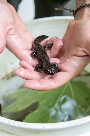
See many more fantastic photos (Study site! Salamanders and trout being measured! and more!) from the Mack Creek vertebrates study at the HJ Andrews Experimental Forest Photo Gallery!
Data exploration
The and_vertebrates data sample is in tidy format,
containing 16 total variables (7 character, 8 numeric, 1 Date). Learn
more about the variables in the data documentation
(?and_vertebrates) and in the original data
package metadata.
glimpse(and_vertebrates)## Rows: 32,209
## Columns: 16
## $ year <dbl> 1987, 1987, 1987, 1987, 1987, 1987, 1987, 1987, 1987, 1987…
## $ sitecode <chr> "MACKCC-L", "MACKCC-L", "MACKCC-L", "MACKCC-L", "MACKCC-L"…
## $ section <chr> "CC", "CC", "CC", "CC", "CC", "CC", "CC", "CC", "CC", "CC"…
## $ reach <chr> "L", "L", "L", "L", "L", "L", "L", "L", "L", "L", "L", "L"…
## $ pass <dbl> 1, 1, 1, 1, 1, 1, 1, 1, 1, 1, 1, 1, 1, 1, 1, 1, 1, 1, 1, 1…
## $ unitnum <dbl> 1, 1, 1, 1, 1, 1, 1, 1, 1, 1, 1, 1, 1, 1, 1, 1, 2, 2, 2, 2…
## $ unittype <chr> "R", "R", "R", "R", "R", "R", "R", "R", "R", "R", "R", "R"…
## $ vert_index <dbl> 1, 2, 3, 4, 5, 6, 7, 8, 9, 10, 11, 12, 13, 14, 15, 16, 1, …
## $ pitnumber <dbl> NA, NA, NA, NA, NA, NA, NA, NA, NA, NA, NA, NA, NA, NA, NA…
## $ species <chr> "Cutthroat trout", "Cutthroat trout", "Cutthroat trout", "…
## $ length_1_mm <dbl> 58, 61, 89, 58, 93, 86, 107, 131, 103, 117, 100, 127, 99, …
## $ length_2_mm <dbl> NA, NA, NA, NA, NA, NA, NA, NA, NA, NA, NA, NA, NA, NA, NA…
## $ weight_g <dbl> 1.75, 1.95, 5.60, 2.15, 6.90, 5.90, 10.50, 20.60, 9.55, 13…
## $ clip <chr> "NONE", "NONE", "NONE", "NONE", "NONE", "NONE", "NONE", "N…
## $ sampledate <date> 1987-10-07, 1987-10-07, 1987-10-07, 1987-10-07, 1987-10-0…
## $ notes <chr> NA, NA, NA, NA, NA, NA, NA, NA, NA, NA, NA, NA, NA, NA, NA…Exploring length-weight relationships
There is opportunity to explore and model the length-weight
relationships for the three species (for example, using the standard
length-weight relationship for fish: \(W =
aL^b\)). Note: only 15 observations in the dataset are Cascade
Torrent Salamanders (compared to 11,758 Coastal Giant Salamanders and
20,433 Coastal Cutthroat Trout). We omit Cascade Torrent Salamanders
throughout this vignette. The length_1_mm variable is the
total or snout-fork length for cutthroat trout (total length from 1987 -
1994; snout-fork length since 1995), and snout-vent length for
salamanders (all in millimeters).
and_vertebrates %>%
filter(species != "Cascade torrent salamander") %>%
ggplot(aes(x = length_1_mm, y = weight_g)) +
  geom_point(aes(color = species)) +
  theme_minimal()
## Warning: Removed 13270 rows containing missing values (`geom_point()`).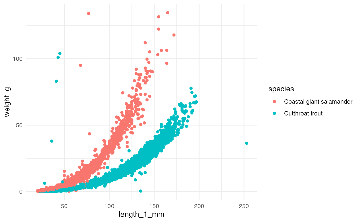
Comparisons by section (clear cut or old growth)
The two sections in the dataset (CC = clear cut circa 1963, OG = upstream 500 year old growth coniferous forest) provide opportunity to explore differences in vertebrate biomass and abundance in the separate sections. Again, we omit Cascade Torrent Salamanders here due to the very small sample size (n = 15) relative to the other species.
Vertebrate abundance by year and section
We can explore abundance (counts) of Coastal Cutthroat Trout and Coastal Giant Salamanders in clear cut (CC) and old growth (OG) forest sections of the creek.
vert_counts <- and_vertebrates %>%
  filter(species != "Cascade torrent salamander") %>%
  drop_na(year, species, section) %>%
  count(year, species, section)
ggplot(data = vert_counts, aes(x = year, y = n)) +
  geom_line(aes(color = section)) +
  geom_point(aes(color = section)) +
  theme_minimal() +
  facet_wrap(~species)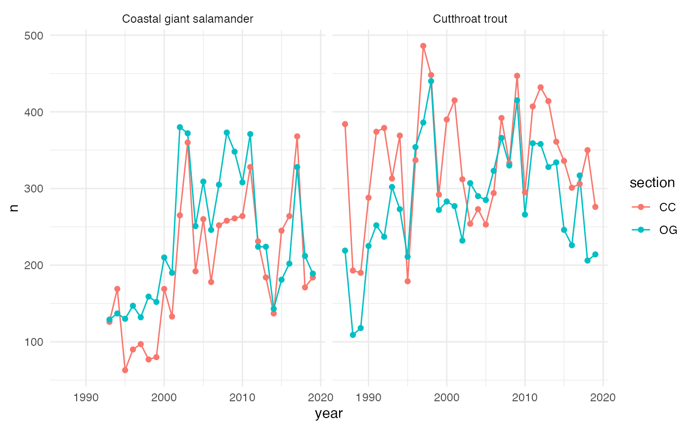
We can also explore the correlation in abundance (or biomass) in old growth and clear cut sections of the creek.
vert_counts_wide <- vert_counts %>%
  pivot_wider(names_from = section, values_from = n)

ggplot(data = vert_counts_wide, aes(x = CC, y = OG)) +
  geom_point() +
  theme_minimal() +
  facet_wrap(~species, scales = "free")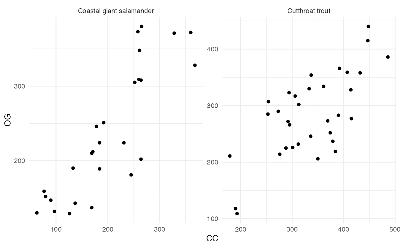
Abundance and size by channel unit
The variable unittype contains channel unit
classification (e.g. “cascade”, “pool”, “rapid”, etc.). See the data
sample documentation (?and_vertebrates) to see the other
classification levels.
For example, just considering cutthroat trout, in which channel classification do they tend to be most abundant?
and_vertebrates %>%
  filter(species == "Cutthroat trout") %>%
  drop_na(unittype) %>%
  count(unittype) %>%
  mutate(unittype = fct_reorder(unittype, n)) %>%
  ggplot(aes(y = unittype, x = n)) +
  geom_col() +
  theme_minimal()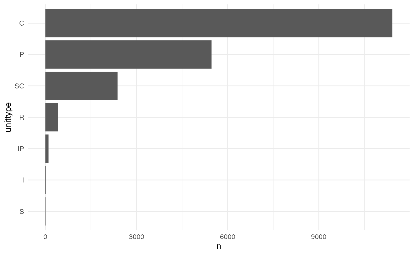
We can see that for Coastal Cutthroat Trout, fish are most abundant in cascade (C), pool (P) and side channel (SC) habitats.
Then we might ask: for those three unit classifications (cascade, pool, and channel), how do cutthroat trout sizes compare?
and_vertebrates %>%
  filter(species == "Cutthroat trout",
         unittype %in% c("C", "P", "SC")) %>%
  ggplot(aes(x = length_1_mm)) +
  geom_histogram() +
  facet_wrap(~unittype, ncol = 1)
## `stat_bin()` using `bins = 30`. Pick better value with `binwidth`.## Warning: Removed 5 rows containing non-finite values (`stat_bin()`).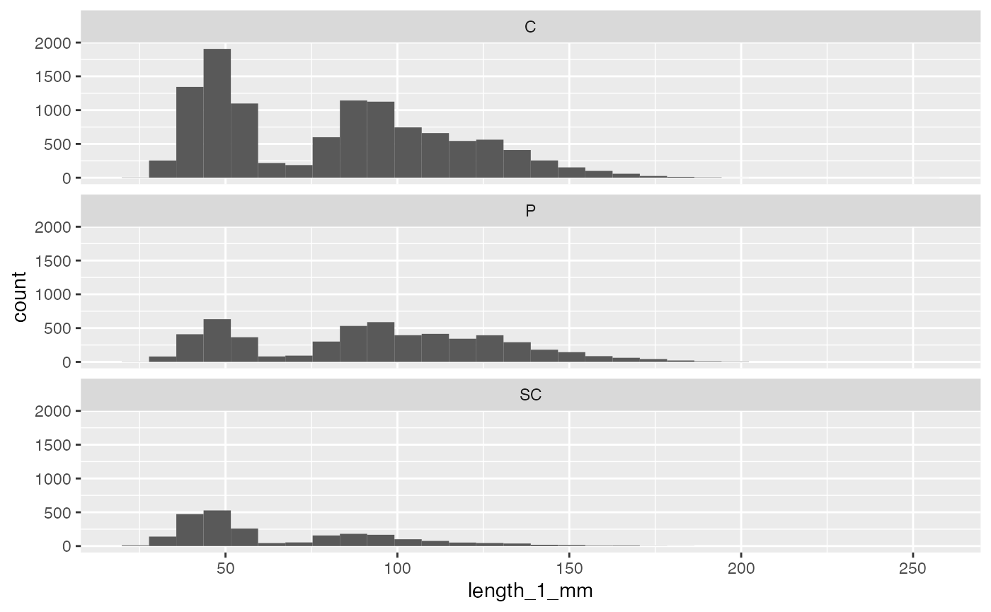
Other things to explore
- Further explore differences in abundance, size and biomass for trout and salamanders by creek sections (previously harvested, or old growth) or channel unit classification (e.g. cascade versus pool)
- Use tag number (variable
pitnumber) to explore growth of unique individuals - Estimate parameters of the length-weight relationship for fish and salamanders
Acknowledgements
Thank you to: original data collectors and researchers (see citation below), and Dr. Brooke Penaluna (Fish Biologist, HJ Andrews Experimental Forest Lead Scientist) for feedback and corrections!
Citations
Kaylor, M.J. and D.R. Warren. 2017. Linking riparian shade and the legacies of forest management to fish and vertebrate biomass in forested streams. Ecosphere 8(6). https://doi.org/10.1002/ecs2.1845
Gregory, S.V. and I. Arismendi. 2020. Aquatic Vertebrate Population Study in Mack Creek, Andrews Experimental Forest, 1987 to present ver 14. Environmental Data Initiative. https://doi.org/10.6073/pasta/7c78d662e847cdbe33584add8f809165 (Accessed 2020-10-09).
How we processed the raw data
Download the raw data from EDI.org
library(tidyverse)
library(lubridate)
library(janitor)
library(usethis)
library(metajam)

and_url <- "https://portal.edirepository.org/nis/dataviewer?packageid=knb-lter-and.4027.14&entityid=5b18ded1cd996f5e8d361a9275a600cf"
and_download <- download_d1_data(data_url = and_url, path = tempdir(), dir_name = "and")
Data cleaning
# Read in data
and_files <- read_d1_files(and_download)
and_data <- and_files$data

# Basic cleaning

and_vertebrates <- and_data %>%
  janitor::clean_names() %>%
  rename(length_1_mm = length1,
         length_2_mm = length2,
         weight_g = weight) %>%
  select(-dbcode, -entity) %>%
  mutate(species = case_when(
    species == "ONCL" ~ "Cutthroat trout",
    species == "DITE" ~ "Coastal giant salamander",
    species == "RHOL" ~ "Cascade torrent salamander",
    TRUE ~ species
  ))