ntl_icecover - North Temperate Lakes Ice Cover (NTL) • lterdatasampler

Dataset sample used

ntl_icecover
ntl_airtemp

Introduction

The vignette highlights:

How to explore time-series trends
How to combine group_by() with summarise() and mutate()
How to join two datasets with left_join()
An example of computing standardized anomalies on long time-series
Use of the patchwork package to combine plots into one figure

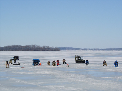
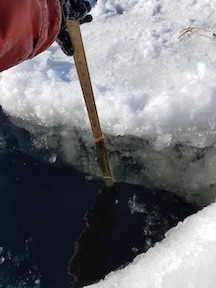
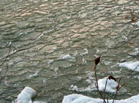
According to the EPA, lake ice duration can be an indicator of climate change. This is because lake ice is dependent on several environmental factors, so changes in these factors will influence the formation of ice on top of lakes. As a result, the study and analysis of lake ice formation can inform scientists about how quickly the climate is changing, and are critical to minimizing disruptions to lake ecosystems. We can examine the ice duration of Lake Mendota, Lake Monona, and Lake Wingra, three lakes in the Madison, WI area.

North Temperate Lakes, LTER CC BY-SA 4.0

Ice measurement Mendota lake, Photo E. Whitaker

Fun Fact:

Did you know that Joni Mitchell’s album “Hejira” art is her skating on Lake Mendota in 1976 !? https://wisconsinlife.org/story/joni-mitchell-skates-on-lake-mendota-and-into-music-history/

Data Exploration

library(lterdatasampler)
library(tidyverse)
library(lubridate)
library(patchwork)

Ice Cover Duration Data

head(ntl_icecover)

## # A tibble: 6 × 5
##   lakeid       ice_on     ice_off    ice_duration  year
##   <fct>        <date>     <date>            <dbl> <dbl>
## 1 Lake Mendota NA         1853-04-05           NA  1852
## 2 Lake Mendota 1853-12-27 NA                   NA  1853
## 3 Lake Mendota 1855-12-18 1856-04-14          118  1855
## 4 Lake Mendota 1856-12-06 1857-05-06          151  1856
## 5 Lake Mendota 1857-11-25 1858-03-26          121  1857
## 6 Lake Mendota 1858-12-08 1859-03-14           96  1858

Note that the tidyverse also provides glimpse() for a quick view of a dataset:

glimpse(ntl_icecover)

## Rows: 334
## Columns: 5
## $ lakeid       <fct> Lake Mendota, Lake Mendota, Lake Mendota, Lake Mendota, L…
## $ ice_on       <date> NA, 1853-12-27, 1855-12-18, 1856-12-06, 1857-11-25, 1858…
## $ ice_off      <date> 1853-04-05, NA, 1856-04-14, 1857-05-06, 1858-03-26, 1859…
## $ ice_duration <dbl> NA, NA, 118, 151, 121, 96, 110, 117, 132, 104, 125, 118, …
## $ year         <dbl> 1852, 1853, 1855, 1856, 1857, 1858, 1859, 1860, 1861, 186…

Now let’s explore the data visually. We can explore the data distribution in the different lakes using a box plot

lake_ice <-
  ggplot(data = ntl_icecover %>% filter(!is.na(ice_duration)), aes(x = lakeid, y = ice_duration)) +
  geom_boxplot(aes(color = lakeid, shape = lakeid),
               alpha = 0.8,
               width = 0.5) +
  theme_minimal() +
  labs(
    title = "Ice Duration of Lakes in the Madison, WI Area",
    y = "Ice Duration (Days)",
    x = "Lake",
    subtitle = "North Temperate Lakes LTER"
  ) +
  geom_jitter(
    aes(color = lakeid),
    alpha = 0.5,
    show.legend = FALSE,
    position = position_jitter(width = 0.2, seed = 0)
  )

lake_ice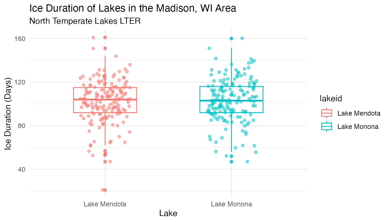

Looking at the time-series across the different lakes:

ice_duration <-
  ggplot(data = ntl_icecover, aes(x = year)) +
  geom_line(aes(y = ice_duration, color = lakeid), alpha = 0.7) +
  theme_minimal() +
  labs(x = "Year", y = "Ice Duration (Days)", title = "Ice Duration of Lakes in the Madison, WI Area", subtitle = "North Temperate Lakes LTER")

ice_duration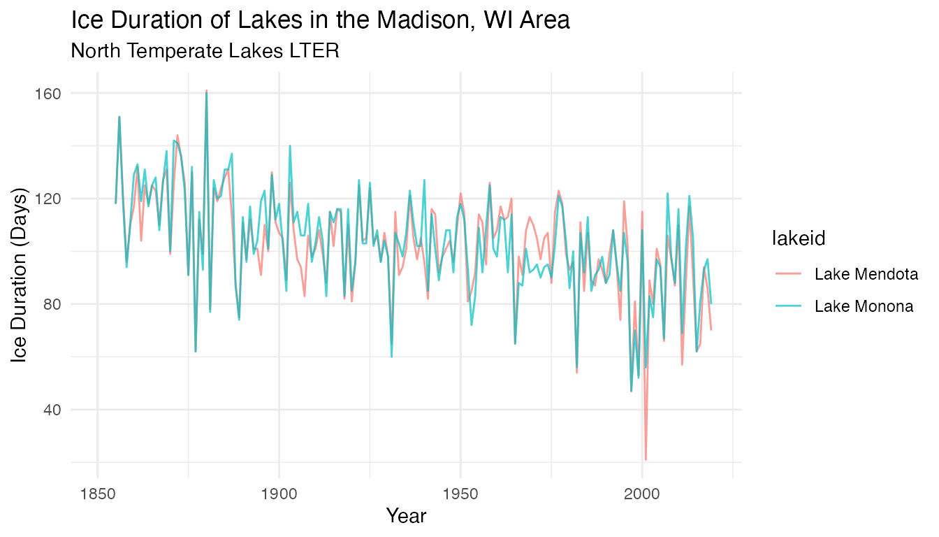

Box plots and time series plots reveal similarities across the 2 lakes. What does the trend look like for average ice cover duration in the region, based on data for the 2 lakes here?

ntl_icecover_avg <- ntl_icecover %>%
  drop_na(ice_duration) %>% 
  group_by(year) %>%
  summarise(ice_duration = mean(ice_duration)) %>%
  rename(avg_ice_duration = ice_duration)

ntl_icecover_avg

## # A tibble: 166 × 2
##     year avg_ice_duration
##    <dbl>            <dbl>
##  1  1851             103 
##  2  1855             118 
##  3  1856             151 
##  4  1857             120 
##  5  1858              95 
##  6  1859             110.
##  7  1860             123 
##  8  1861             132.
##  9  1862             112.
## 10  1863             128 
## # ℹ 156 more rows

Time Series Plot:

avg_ice_duration <-
  ggplot(data = ntl_icecover_avg %>% filter(!is.na(avg_ice_duration)), aes(x = year, y = avg_ice_duration)) +
  geom_line(alpha = 0.7) +
  theme_minimal() +
  geom_smooth(
    method = lm,
    se = FALSE,
    color = "blue",
    linetype = "dashed"
  ) + 
  labs(y = "Ice Duration (Days)", x = "Year", title = "Average Ice Duration", subtitle = "North Temperate Lakes LTER")

avg_ice_duration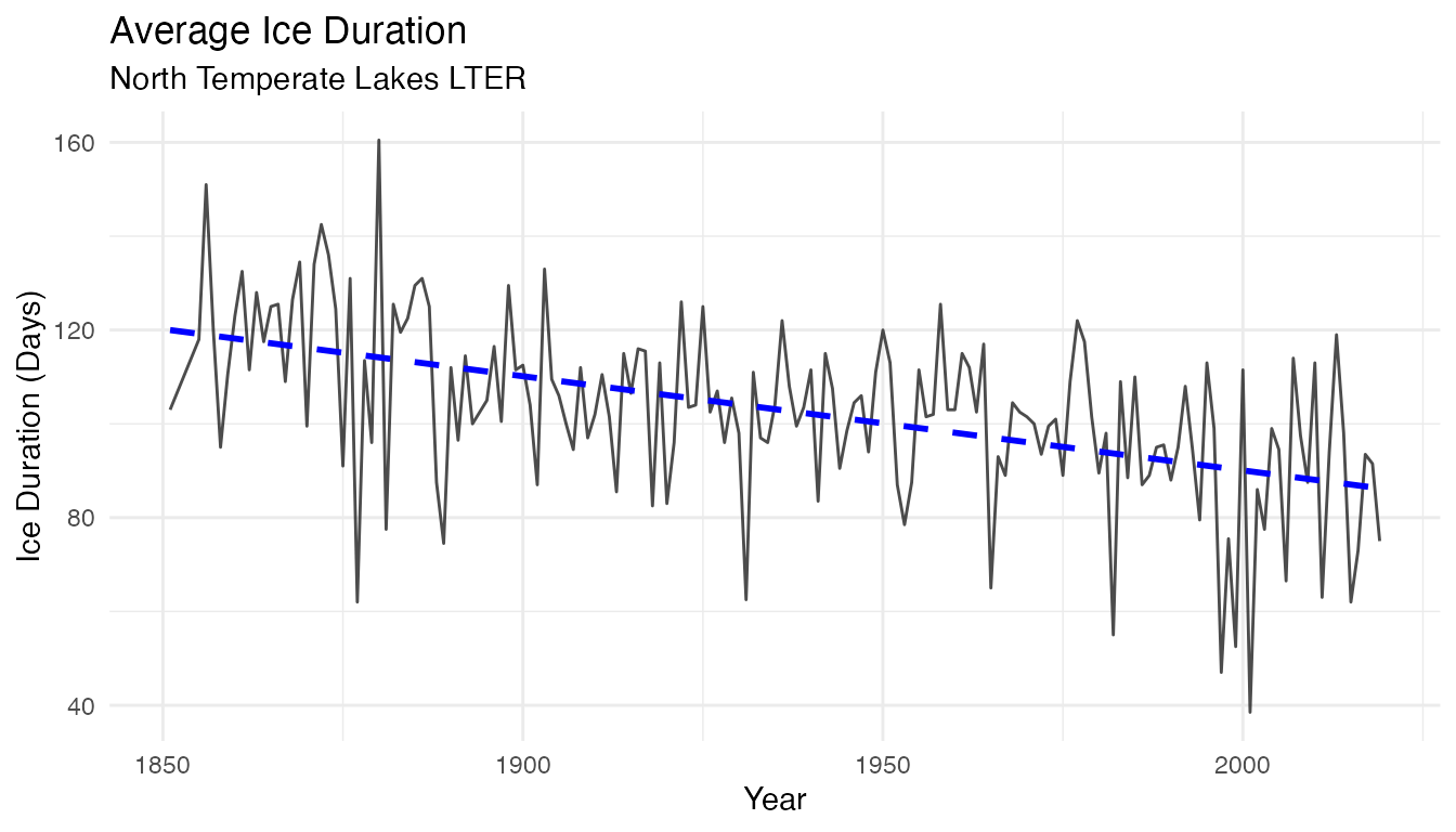

Over the 168 years of this time series, the average ice duration in North Temperate Lakes is decreasing from about 120 days to about 80 days. Let us investigate a little more what could be the environmental factors are influencing this change!

Pancake ice formed near shore when early ice is broken by wave action, Lake Mendota, Dec. 2003; Photo: J. Magnuson

Research suggests that mean annual temperature is one of the primary factors that alter lake ice formation. We can look at the temperature data of Madison, WI found in ntl_airtemp to see if there is a corresponding change in climate that may have influenced the change in ice duration.

Note that according to the original metadata: “Daily temperature data prior to 1884 were estimated from 3 times per day sampling and biases are expected and should not be comparable with data after that time.”

Air Temperature Data

head(ntl_airtemp)

## # A tibble: 6 × 3
##   sampledate  year ave_air_temp_adjusted
##   <date>     <dbl>                 <dbl>
## 1 1870-06-05  1870                  20  
## 2 1870-06-06  1870                  18.3
## 3 1870-06-07  1870                  17.5
## 4 1870-06-09  1870                  13.3
## 5 1870-06-10  1870                  13.9
## 6 1870-06-11  1870                  15

We can compute the mean annual air temperature using group_by and summarise:

ntl_airtemp_avg <- ntl_airtemp %>% 
  filter(year > 1884) %>%   # filter out the known biased data
  group_by(year) %>% 
  summarise(avg_air_temp_adjusted = mean(ave_air_temp_adjusted, na.rm=TRUE))

ntl_airtemp_avg

## # A tibble: 135 × 2
##     year avg_air_temp_adjusted
##    <dbl>                 <dbl>
##  1  1885                  5.04
##  2  1886                  6.65
##  3  1887                  6.64
##  4  1888                  5.59
##  5  1889                  7.44
##  6  1890                  7.25
##  7  1891                  7.18
##  8  1892                  6.02
##  9  1893                  5.87
## 10  1894                  8.21
## # ℹ 125 more rows

Time Series Plot:

temp_plot <-
  ggplot(data = ntl_airtemp_avg,
         aes(x = year, y = avg_air_temp_adjusted)) +
  geom_line(alpha = 0.7) +
  theme_minimal() +
  geom_smooth(
    method = lm,
    se = FALSE,
    color = "blue",
    linetype = "dashed"
  ) +
  labs(y = "Mean Air Temperature Nov-April (Celsius)", x = "Year", title = "Mean Annual Temperature", subtitle = "Madison, WI")

temp_plot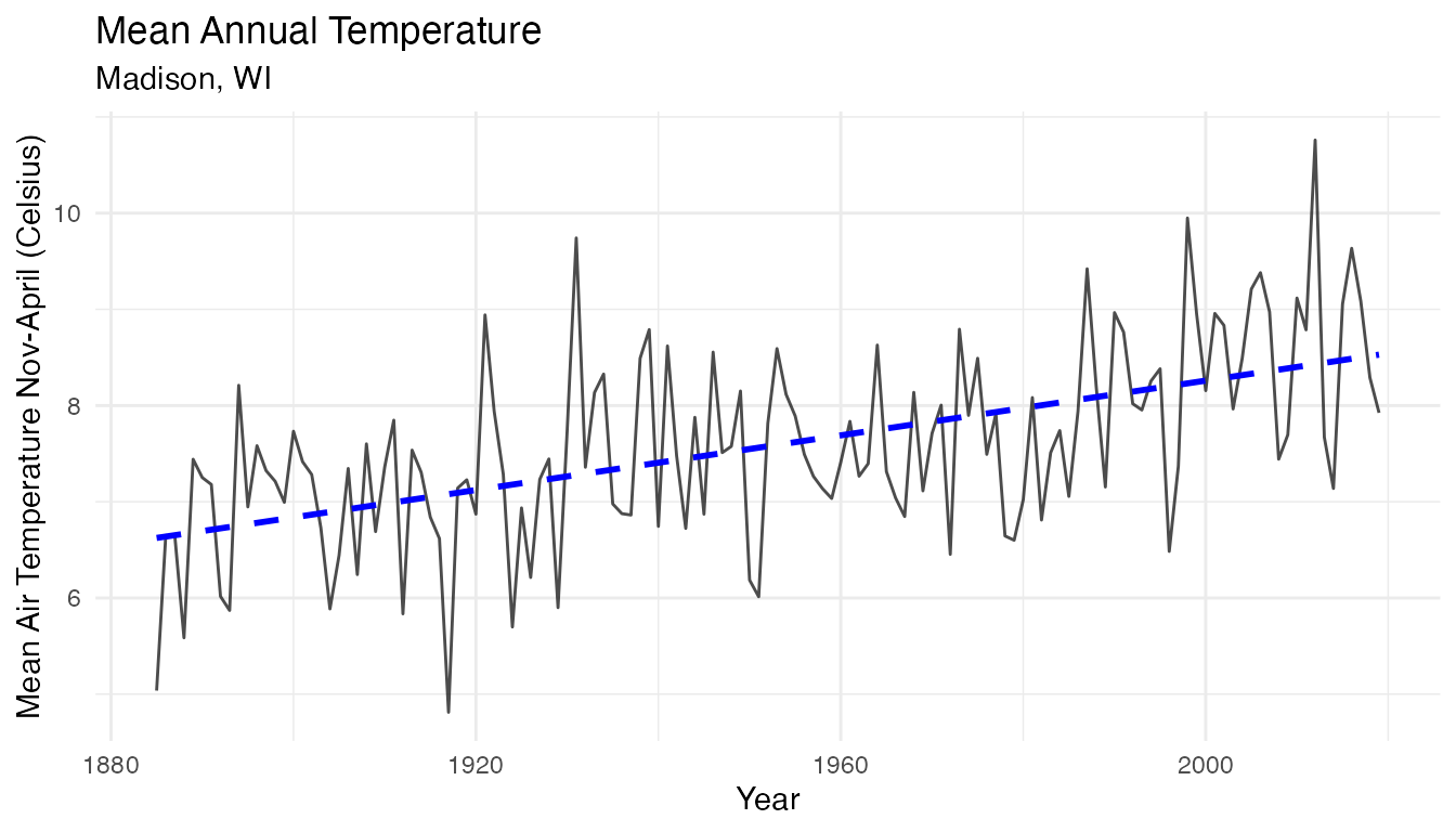

There is an upward trend in the mean annual air temperature. Let’s investigate potential relationships between air temperature and lake ice cover duration.

Investigate the relationship between ice cover duration and air temperature

To compare the ice cover duration and temperature data directly, the ntl_airtemp and ntl_icecover datasets can be joined. Since lake freezing is mostly impacted by Fall and Spring air temperatures, we will first compute the mean temperature from Nov to April (next year) to best capture the potential relationship:

# Add a column to group the Fall and Spring season into a same year, similarly to what is done when defining hydrological year
ntl_airtemp_hydro <- ntl_airtemp %>%
  mutate(hydroyear = if_else(month(sampledate) < 10, year-1, year))

# Compute the average air temperature from Nov to April
ntl_airtemp_avg_winter <-  ntl_airtemp_hydro %>%
  filter(month(sampledate) %in% c(11:12,1:4)) %>% # filter the months from Nov to April
  group_by(hydroyear) %>%
  summarise(avg_air_temp_adjusted = mean(ave_air_temp_adjusted))

Let us plot the average air temperature time-series computed from the cold season:

temp_plot <-
  ggplot(data = ntl_airtemp_avg_winter %>% filter(!is.na(avg_air_temp_adjusted)),
         aes(x = hydroyear, y = avg_air_temp_adjusted)) +
  geom_line(alpha = 0.7) +
  theme_minimal() +
  geom_smooth(
    method = lm,
    se = FALSE,
    color = "blue",
    linetype = "dashed"
  ) +
  labs(y = "Mean Air Temperature Nov-April (Celsius)", x = "Year", title = "Cold Season (Nov to Apr) Mean Annual Temperature", subtitle = "Madison, WI")

temp_plot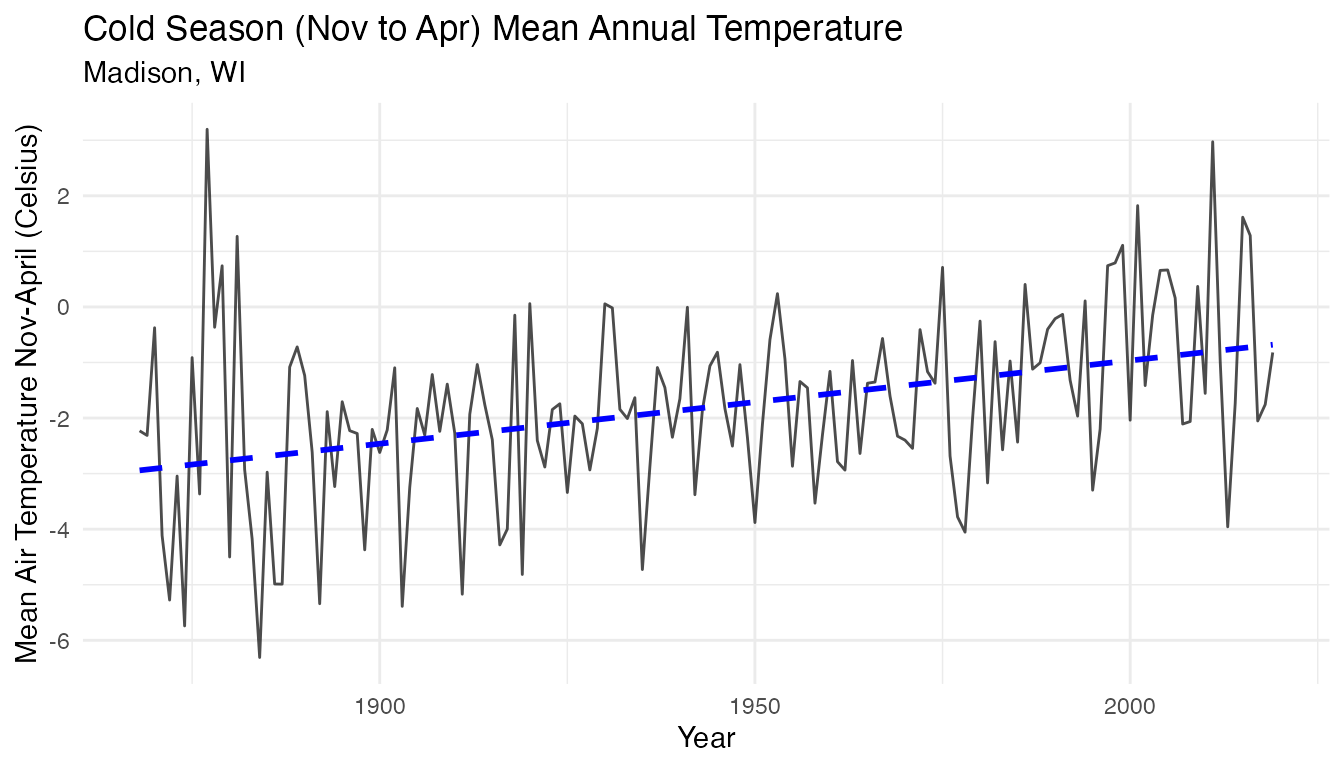

To further investigate the relationship between the air temperature during the cold season and the ice cover duration, we can join the two datasets together using left_join:

ntl_joined_avg <- ntl_icecover_avg  %>%
  left_join(by = c("year" = "hydroyear"), ntl_airtemp_avg_winter)

ntl_joined_avg

## # A tibble: 166 × 3
##     year avg_ice_duration avg_air_temp_adjusted
##    <dbl>            <dbl>                 <dbl>
##  1  1851             103                     NA
##  2  1855             118                     NA
##  3  1856             151                     NA
##  4  1857             120                     NA
##  5  1858              95                     NA
##  6  1859             110.                    NA
##  7  1860             123                     NA
##  8  1861             132.                    NA
##  9  1862             112.                    NA
## 10  1863             128                     NA
## # ℹ 156 more rows

Plot the average air temperature against the average ice cover duration:

scatter <-
  ggplot(data = ntl_joined_avg ,
       aes(y = avg_ice_duration, x = avg_air_temp_adjusted)) + geom_point(alpha = 0.8) +
  theme_minimal() +
  labs(
    title = "Cold Season Mean Air Temperature and Ice Duration of Lakes",
    y = "Ice Duration (Days)",
    x = "Mean Air Temperature Nov-April (Celsius)",
    subtitle = "North Temperate Lakes LTER"
  ) +
  geom_smooth(
    method = "lm",
    color = "black",
    se = FALSE,
    size = 0.3
  )
scatter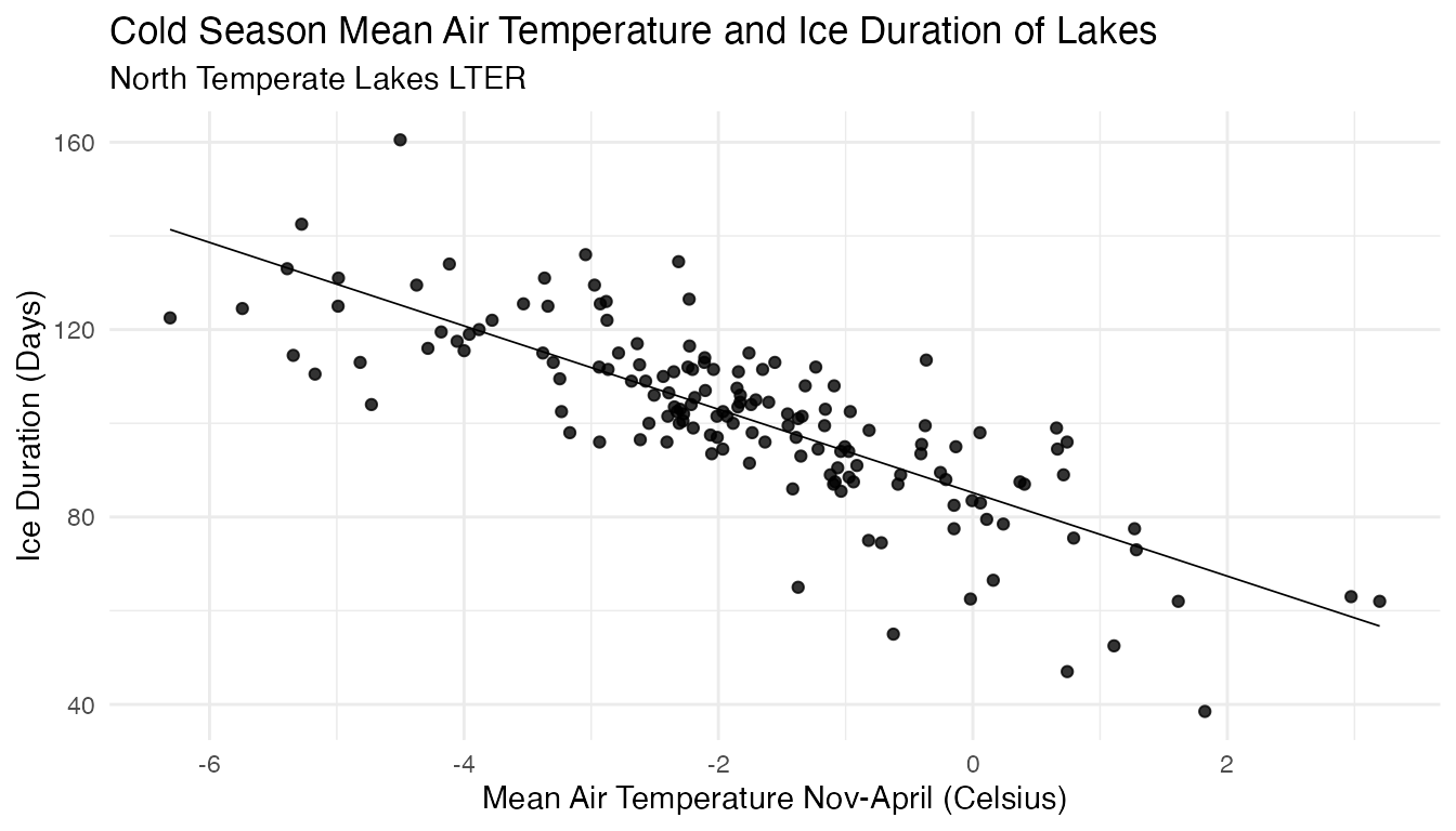

There is a negative correlation between the mean air temperature from November to April and the amount of time that each lake was frozen. This means that as temperature increases, the ice duration decreases.

Standardized Anomalies

Now let’s investigate how this relationship evolves over time. To compare the temperature with the ice duration on a time-series plot on a similar scale we are going to compute standardized anomalies for both parameters. We are going to split the time-series in two parts. The first 30 years will be used to compute the climatological reference (mean and standard deviation), that we will use to compare the other years against. Since the earliest year of observation for ice duration was 1851, and the earliest year of observation for temperature was 1869, we opted to compute the climatological references from 1870 to 1900.

In this example, the standardized anomalies for the temperature (and ice cover duration) are computed as follow:

\(A_{y_{stand}} = (T_{y} - \overline{T}_{clim}) / T_{SD_{clim}}\)

Where:

\(A_{y_{stand}}\) = Standardized anomalies
\(T_{y}\) = mean temperature for a specific cold season
\(\overline{T}_{clim}\) = Mean temperature from 1870 to 1900
\(T_{SD_{clim}}\) = Standard deviation for temperature from 1870 to 1900

Air Temperature Climatologies

Let us start with computing the climatologies and standardized anomalies for the air temperature:

# Using the first 30 years to compute the yearly climatologies
ntl_airtemp_clim <- ntl_airtemp_avg_winter %>%
  filter(hydroyear > 1869 & hydroyear < 1901) %>%   # taking the first 30 years of common data
  summarise(clim_winter_mean_airtemp = mean(avg_air_temp_adjusted, na.rm=TRUE),  # computing the climatologies
            clim_winter_sd_airtemp = sd(avg_air_temp_adjusted, na.rm=TRUE)) %>%
  bind_cols(filter(ntl_airtemp_avg_winter,hydroyear > 1900), .) %>%  # Adding the climatology columns to the second part of the time-series
  mutate(standardized_anomalies_airtemp = (avg_air_temp_adjusted - clim_winter_mean_airtemp) / clim_winter_sd_airtemp)  # computing the standardized anomalies

Let’s plot the standardized anomalies time-series:

temp_plot_airtemp_anomalies <-
  ggplot(data = ntl_airtemp_clim,
         aes(x = hydroyear, y = standardized_anomalies_airtemp)) +
  geom_bar(stat = "identity", show.legend = FALSE) +
  theme_minimal() +
  # scale_x_date(date_breaks = "year", date_labels = "%b") +
  geom_smooth(
    method = lm,
    se = FALSE,
    color = "blue",
    linetype = "dashed"
  ) +
  labs(y = "Standaradized Anomalies", x = "Year", title = "Air temperature standaradized anomalies", subtitle = "Madison, WI")

temp_plot_airtemp_anomalies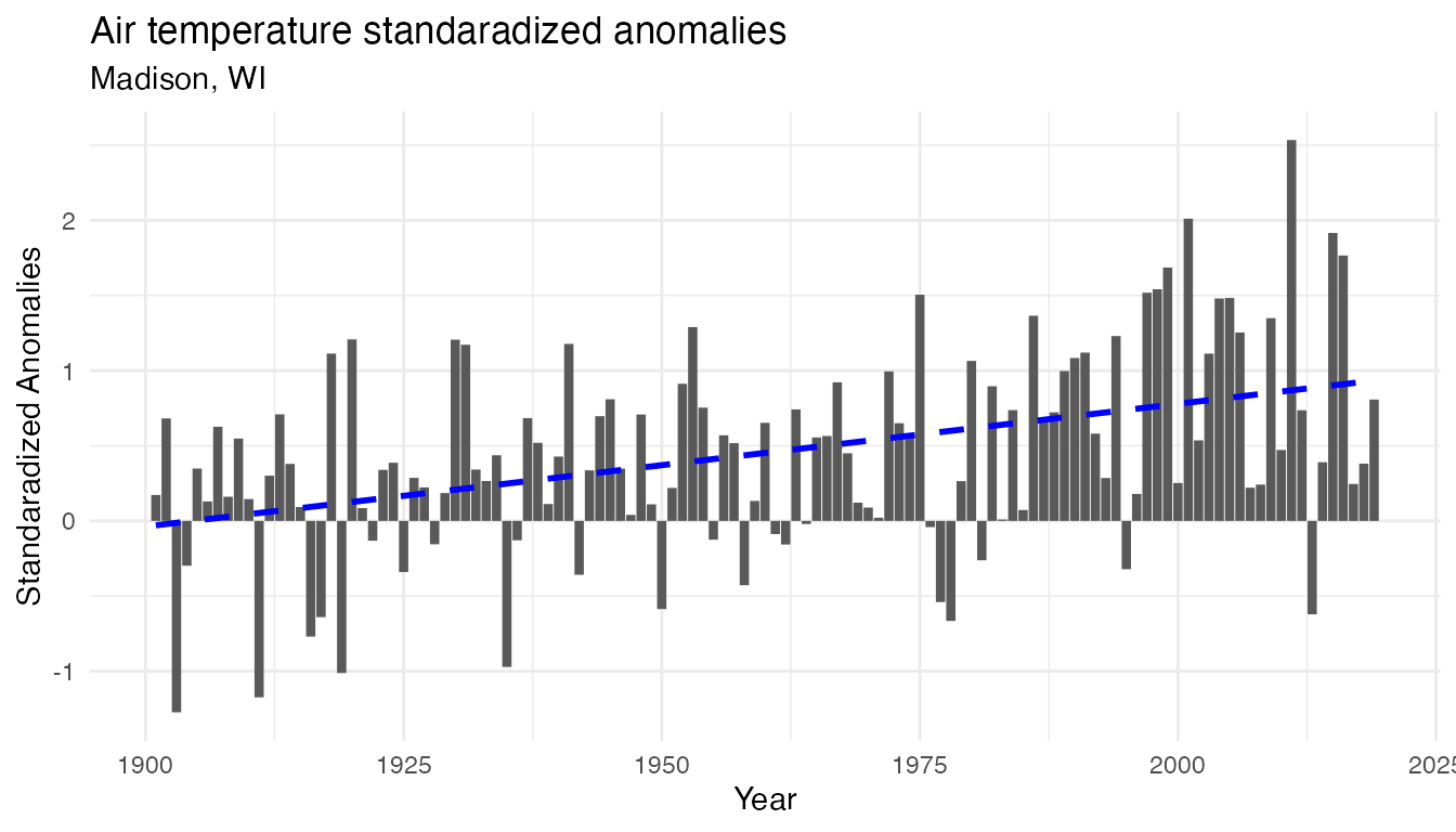

Ice Cover Duration Climatologies

Now doing the same computations for the ice cover duration:

# Using the first 30 years to compute the yearly climatologies
ntl_iceduration_clim_30first <- ntl_icecover_avg %>%
  filter(year > 1869 & year < 1901) %>%  # taking the first 30 years of common data
  summarise(clim_mean_iceduration = mean(avg_ice_duration, na.rm=TRUE),  # computing the climatologies
         clim_sd_iceduration = sd(avg_ice_duration, na.rm=TRUE)) 

# compute the yearly standardized anomalies
ntl_iceduration_clim <- ntl_icecover %>%
  filter(year > 1900) %>%   # using the following years of the time series
  add_column(clim_mean_iceduration = ntl_iceduration_clim_30first$clim_mean_iceduration,
             clim_sd_iceduration = ntl_iceduration_clim_30first$clim_sd_iceduration) %>%
  mutate(standardized_anomalies_iceduration = (ice_duration - clim_mean_iceduration) / clim_sd_iceduration) # computing the standardized anomalies

Let’s plot the standardized anomalies time-series:

temp_plot_iceduration_anomalies <-
  ggplot(data = ntl_iceduration_clim,
         aes(x = year, y = standardized_anomalies_iceduration)) +
  geom_bar(stat = "identity", show.legend = FALSE) +
  theme_minimal() +
  # scale_x_date(date_breaks = "year", date_labels = "%b") +
  geom_smooth(
    method = lm,
    se = FALSE,
    color = "blue",
    linetype = "dashed"
  ) +
  labs(y = "Standaradized Anomalies", x = "Year", title = "Ice cover duration standaradized anomalies", subtitle = "North Temperate Lakes LTER")

temp_plot_iceduration_anomalies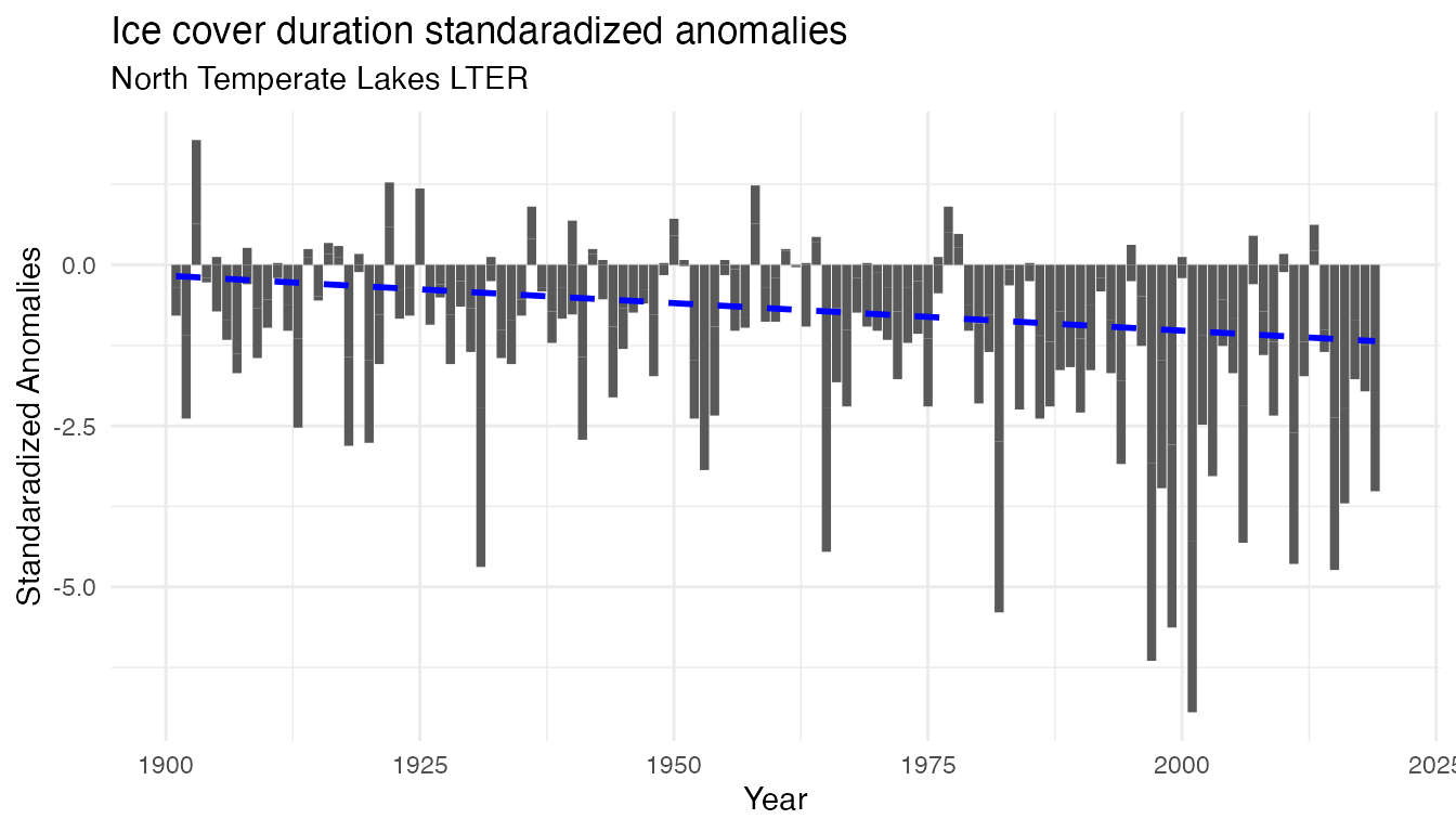

Using the patchwork package, it is very easy to combine graphs together: just add them!!

temp_plot_airtemp_anomalies + temp_plot_iceduration_anomalies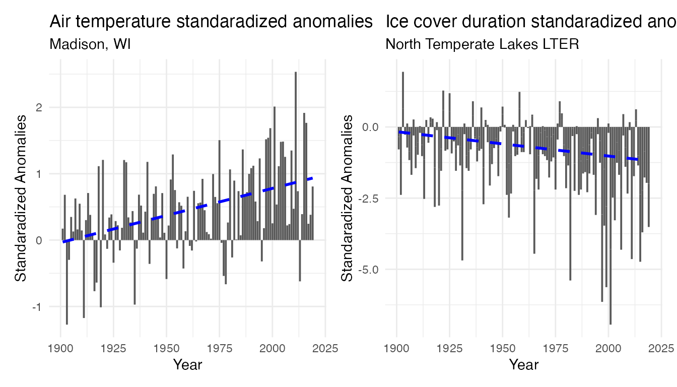

or try vertically:

temp_plot_airtemp_anomalies / temp_plot_iceduration_anomalies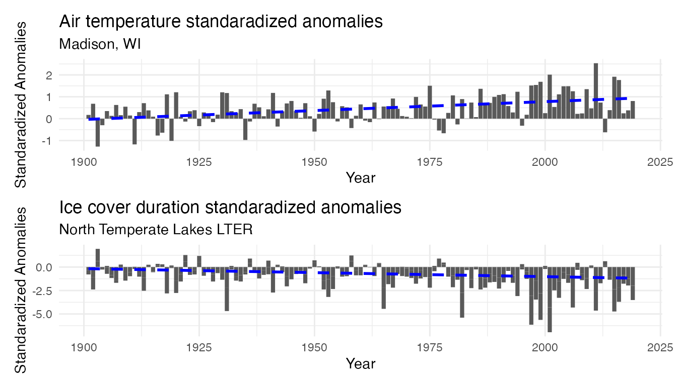

Note the difference of scale on the y-axis. However in both time series, there is an increase in anomalies (both in frequency and intensity) over time, suggesting the recent year are more consistently warmer and with shorter period with frozen lakes

Other things to explore:

How are the freezing starting date and melting date changing over time?
How does interpretation change with different methods / visualizations of smoothing (e.g. moving average)
Predictions of ice cover duration in the future
Comparison of how those predictions change if you pick a longer or shorter dataset (e.g. how does the coefficient compare if you use all of the data, versus just data since ~1975?)
See the last citation below for more ideas!

Aknowledgement

Thank you to Hilary Dugan, Corinna Gries and John Magnuson for their inputs while developing this vignette. Thank you also go to Adhitya Logan for his extra work on this vignette.

Citation

Anderson, L. and D. Robertson. 2020. Madison Wisconsin Daily Meteorological Data 1869 - current ver 32. Environmental Data Initiative. https://doi.org/10.6073/pasta/e3ff85971d817e9898bb8a83fb4c3a8b (Accessed 2021-03-08).

Magnuson, J.J., S.R. Carpenter, and E.H. Stanley. 2021. North Temperate Lakes LTER: Ice Duration - Madison Lakes Area 1853 - current ver 35. Environmental Data Initiative. https://doi.org/10.6073/pasta/ab31f2489ee436beb73fc8f1d0213d97 (Accessed 2021-03-08).

Magnuson, J.J. 2021. Seeing the invisible present and place: from years to centuries with lake ice from Wisconsin to the Northern Hemisphere. Chapter 9 (243- 277) in R. B. Waide and S. E. Kingsland [eds]. The Challenges of Long Term Ecological Research: A Historical Analysis. Springer, Archimedes Series #59. https://doi.org/10.1007/978-3-030-66933-1_9 (Accessed 2022-02-14).

How we processed the raw data

Ice Cover

Download the raw data from EDI.org

library(usethis)
library(metajam)
library(tidyverse)
library(janitor)

# North Temperate Lakes LTER: Ice Duration - Madison Lakes Area 1853 - current
# Main URL: https://portal.edirepository.org/nis/mapbrowse?scope=knb-lter-ntl&identifier=33&revision=35
# Save link location for the data package:
ntl_url <-
  "https://portal.edirepository.org/nis/dataviewer?packageid=knb-lter-ntl.33.35&entityid=f5bc02452cafcd461c49bd7429d8b40c"

# Download the data package with metajam
ntl_download <-
  download_d1_data(data_url = ntl_url, path = tempdir())

Data Cleaning

# Read in data
ntl_files <- read_d1_files(ntl_download)
ntl_ice_raw <- ntl_files$data

# Basic cleaning
ntl_icecover <- ntl_ice_raw %>%
  select(-iceon, -iceoff, -season) %>%
  rename(year = year4) %>%
  mutate(
    lakeid = recode(
      lakeid,
      "ME" = "Lake Mendota",
      "MO" = "Lake Monona",
      "WI" = "Lake Wingra"
    ),
    year = as.numeric(year),
    ice_duration = as.numeric(ice_duration),
    ice_on = as.Date(ice_on),
    ice_off = as.Date(ice_off),
    lakeid = as.factor(lakeid),
    ice_duration = replace(ice_duration, which(ice_duration < 0), NA) # change values of -999 to NA
  ) %>%
  filter(lakeid != "Lake Wingra") %>% # too many missing data and longer ice cover duration
  clean_names() # makes headers formatting more consistent

Air Temperature

Download the raw data from EDI.org

library(usethis)
library(metajam)
library(tidyverse)
library(janitor)

# Madison Wisconsin Daily Meteorological Data 1869 - current
# Main URL: https://portal.edirepository.org/nis/mapbrowse?packageid=knb-lter-ntl.20.32
ntl_temps_url <-
  "https://portal.edirepository.org/nis/dataviewer?packageid=knb-lter-ntl.20.32&entityid=3c7ddd692d3ac8e90bf2954a16b39e89"

# Download the data package with metajam
ntl_temps_download <-
  download_d1_data(data_url = ntl_temps_url, path = tempdir())

Data Cleaning

# Read in data
ntl_temps_files <- read_d1_files(ntl_temps_download)
ntl_temps_raw <- ntl_temps_files$data

# Basic cleaning
ntl_airtemp <- ntl_temps_raw %>%
  select(sampledate, year4, ave_air_temp_adjusted) %>%
  rename(year = year4) %>%
  clean_names()

ntl_icecover - North Temperate Lakes Ice Cover (NTL)

Comparing Temperatures and Lake Ice Duration in Madison, WI since the 19th Century

Dataset sample used

Introduction

Data Exploration

Ice Cover Duration Data

Air Temperature Data

Investigate the relationship between ice cover duration and air temperature

Standardized Anomalies

Air Temperature Climatologies

Ice Cover Duration Climatologies

Other things to explore:

Aknowledgement

Citation

How we processed the raw data

Ice Cover

Download the raw data from EDI.org

Data Cleaning

Air Temperature

Download the raw data from EDI.org

Data Cleaning