arc_weather - Arctic LTER Toolik Field Station (ARC)

Arctic LTER daily weather data from Toolik Field Station

Dataset sample used

• arc_weather

Introduction

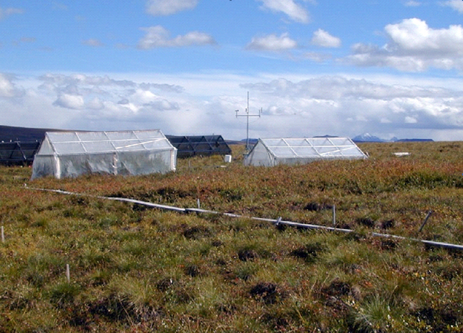
The arc_weather data sample contains selected meteorological records from the Toolik Field Station at Toolik Lake, Alaska, from 1988 - 2018. This data set offers opportunities to explore and wrangle time series data, visualize patterns (e.g. seasonality), and apply different forecasting methods.

LTER research station Toolik Lake, LTER CC BY-SA 4.0

Data exploration

Attach required packages:

library(lterdatasampler)
library(tidyverse)
library(tsibble)
library(feasts)

Here, we highlight daily air temperature (the data sample also contains records for precipitation and wind speed) using functions from the tsibble and feasts R packages (both part of the fantastic tidyverts ecosystem of “tidy tools for time series”).

# Calculate monthly average of daily mean air temperature and convert to tsibble: 
arc_weather_ts <- arc_weather %>% 
  mutate(yr_mo = yearmonth(date)) %>% # Make a column with just month and year from each date
  group_by(yr_mo) %>% # Group by year-month
  summarize(avg_mean_airtemp = mean(mean_airtemp, na.rm = TRUE)) %>% # Find monthly mean air temperature
  as_tsibble(index = yr_mo) # Convert to a tsibble (time series tibble)

# Check out the first 10 lines:
head(arc_weather_ts, 10)

## # A tsibble: 10 x 2 [1M]
##       yr_mo avg_mean_airtemp
##       <mth>            <dbl>
##  1 1988 Jun             9.61
##  2 1988 Jul            12.0 
##  3 1988 Aug             6.96
##  4 1988 Sep            -0.26
##  5 1988 Oct           -16.4 
##  6 1988 Nov           -29.2 
##  7 1988 Dec           -17.1 
##  8 1989 Jan           -29.9 
##  9 1989 Feb            -8.06
## 10 1989 Mar           -19.4

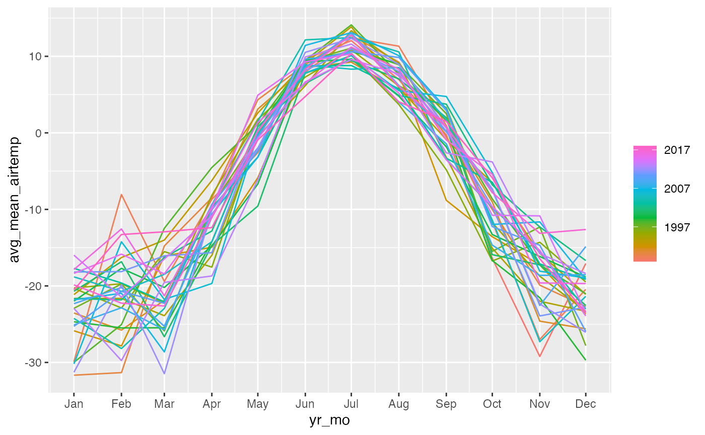
Once the data are converted into a tsibble in the last line above, we can use helpful functions in feasts (like autoplot() and gg_season()) to explore the time series data a bit more.

# Create a line graph of monthly average of mean daily air temperatures:
arc_weather_ts %>% 
  autoplot(avg_mean_airtemp)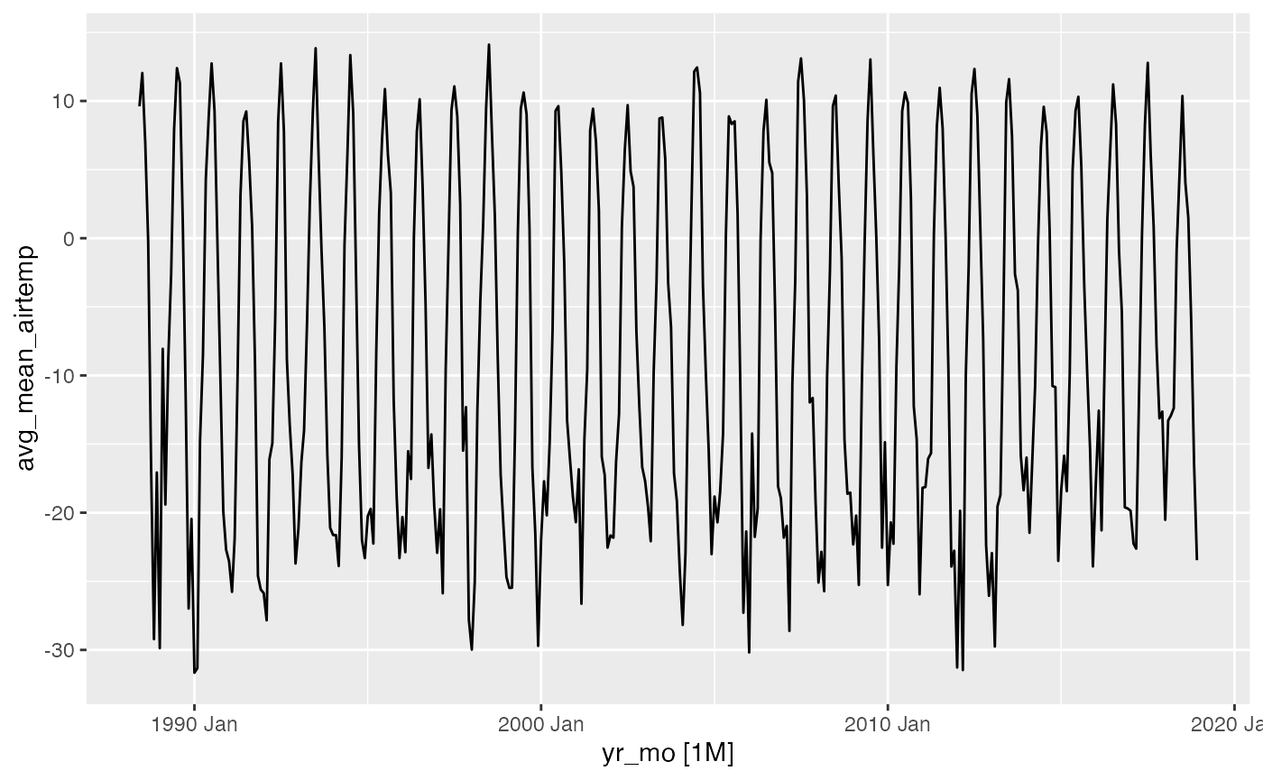

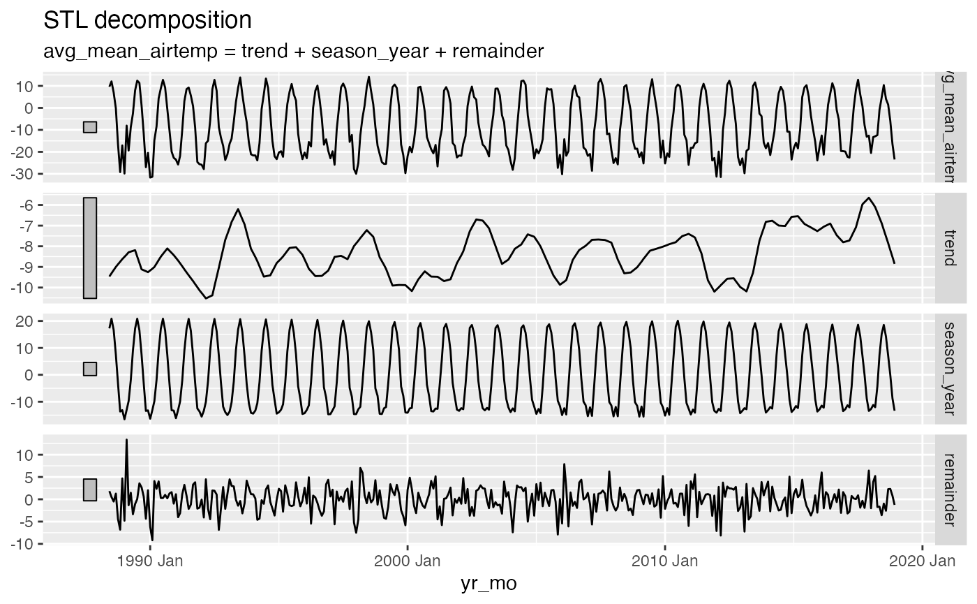
# Create  season plot to explore seasonality: 
arc_weather_ts %>% 
  gg_season(avg_mean_airtemp)

We might want to decompose the time series data to further explore components. See Chapter 3 Time series decomposition in Forecasting: Principles and Practice by Rob J Hyndman and George Athanasopoulos for more information on decomposing time series data.

arc_weather_ts %>% 
  model(STL(avg_mean_airtemp)) %>% 
  components() %>% 
  autoplot()

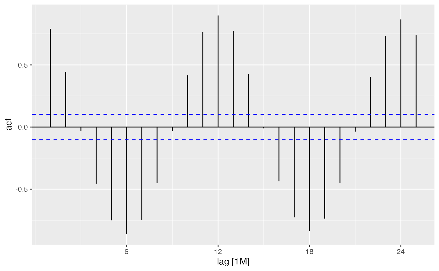
We can also explore autocorrelation:

arc_weather_ts %>% 
  ACF(avg_mean_airtemp) %>% 
  autoplot()

Then you can move on to time series forecasting and further analysis! Have fun with the arc_weather data sample from Arctic LTER.

Acknowledgements

Citation

Shaver, G. 2019. A multi-year DAILY weather file for the Toolik Field Station at Toolik Lake, AK starting 1988 to present. ver 4. Environmental Data Initiative. https://doi.org/10.6073/pasta/ce0f300cdf87ec002909012abefd9c5c (Accessed 2020-07-04).

How we processed the raw data

Download the raw data from EDI.org

library(tidyverse)
library(lubridate)
library(janitor)
library(usethis)
library(metajam)

arc_url <- "https://portal.edirepository.org/nis/dataviewer?packageid=knb-lter-arc.1489.4&entityid=280f9818386cc1abaaa95b638ed079ca"
arc_weather_path <- download_d1_data(data_url = arc_url, path = tempdir())

Data cleaning

# Read that data
# View(stream_chem$attribute_metadata)
arc_weather <- read_d1_files(arc_weather_path, na = c("", "#N/A"))
arc_weather <- arc_weather$data

# Simplify to convert date to class 'date', reduce variables to date, station, mean_airtemp, daily_precip, mean_windspeed:

arc_weather <- arc_weather %>%
  janitor::clean_names() %>%
  dplyr::select(date, station, daily_air_temp_mean_c, daily_precip_total_mm, daily_windsp_mean_msec) %>%
  rename(mean_airtemp = daily_air_temp_mean_c,
         daily_precip = daily_precip_total_mm,
         mean_windspeed = daily_windsp_mean_msec) %>%
  mutate(date = ymd(date)) %>%
  mutate(station = tolower(station)) %>%
  mutate(station = case_when(
    station == "tlkmain" ~ "Toolik Field Station"
  ))