# Note that these lines only need to be run once per computer
## So you can skip this step if you've installed these before
install.packages("vegan")
install.packages("ape")
install.packages("supportR")Multivariate Visualization
Overview
Synthesis projects often eventually want to use multivariate statistics and visualization. This makes a lot of sense when you consider that many synthesis projects eventually have many (many) variables so reducing the dimensionality of the data can be one way of looking at differences that might not be apparent in any variable by itself. Just as univariate statistics are only shallowly discussed in this course, we won’t dive into multivariate statistics here but multivariate visualization (or at least some common methods under that heading) is reasonable to cover in this module.
Learning Objectives
After completing this module you will be able to:
- Define some common multivariate visualization methods
- Describe the similarities/differences between metric and non-metric ordination (methodology and interpretation)
Preparation
This is a “bonus” module and thus was created for asynchronous learners. There is no suggested preparatory work.
Networking Session
This was a bonus module for the 2024-25 cohort and so did not include a networking session.
Needed Packages
If you’d like to follow along with the code chunks included throughout this module, you’ll need to install the following packages:
Ordination
Ordination is the general term for many types of multivariate visualization but typically is used to refer to visualizing a distance or dissimiliarity measure of the data. Such measures collapse multiple columns of response variables into fewer (typically two) index values that are easier to visualize.
This is a common approach particularly in answering questions in community ecology or considering a suite of traits (e.g., life history, landscape, etc.) together. While the math behind reducing the dimensionality of your data is interesting, this module is focused on only the visualization facet of ordination so we’ll avoid deeper discussion of the internal mechanics that underpin ordination.
In order to demonstrate two types of ordination we’ll use a lichen community composition dataset included in the vegan package. However, ordination approaches are most often used on data with multiple groups so we’ll need to make a simulated grouping column to divide the lichen community data.
# Load library
library(vegan)

# Grab data
utils::data("varespec", package = "vegan")

# Create a faux group column
treatment <- c(rep.int("Treatment A", nrow(varespec) / 2),
               rep.int("Treatment B", nrow(varespec) / 2))

# Combine into one dataframe
lichen_df <- cbind(treatment, varespec)

# Check structure of first few columns
str(lichen_df[1:5])
'data.frame': 24 obs. of 5 variables:
$ treatment: chr "Treatment A" "Treatment A" "Treatment A" "Treatment A" ...
$ Callvulg : num 0.55 0.67 0.1 0 0 ...
$ Empenigr : num 11.13 0.17 1.55 15.13 12.68 ...
$ Rhodtome : num 0 0 0 2.42 0 0 1.55 0 0.35 0.07 ...
$ Vaccmyrt : num 0 0.35 0 5.92 0 ...Metric ordinations are typically used when you are concerned with retaining quantitative differences among particular points, even after you’ve collapsed many response variables into just one or two. For example, this is a common approach if you have a table of traits and want to compare the whole set of traits among groups while still being able to interpret the effect of a particular effect on the whole.
Two of the more common methods for metric ordination are Principal Components Analysis (PCA), and Principal Coordinates Analysis (PCoA / “metric multidimensional scaling”). The primary difference is that PCA works on the data directly while PCoA works on a distance matrix of the data. We’ll use PCoA in this example because it is closer analog to the non-metric ordination discussed in the other tab. If the holistic difference among groups is of interest, (rather than metric point-to-point comparisons), consider a non-metric ordination approach.
In order to perform a PCoA ordination we first need to get a distance matrix of our response variables and then we can actually do the PCoA step. The distance matrix can be calculated with the vegdist function from the vegan package and the pcoa function in the ape package can do the actual PCoA.
# Load needed libraries
library(vegan); library(ape)

# Get distance matrix
1lichen_dist <- vegan::vegdist(x = lichen_df[-1], method = "kulczynski")

# Do PCoA
pcoa_points <- ape::pcoa(D = lichen_dist)- 1
-
The
methodargument requires a distance/dissimilarity measure. Note that if you use a non-metric measure (e.g., Bray Curtis, etc.) you lose many of the advantages conferred by using a metric ordination approach.
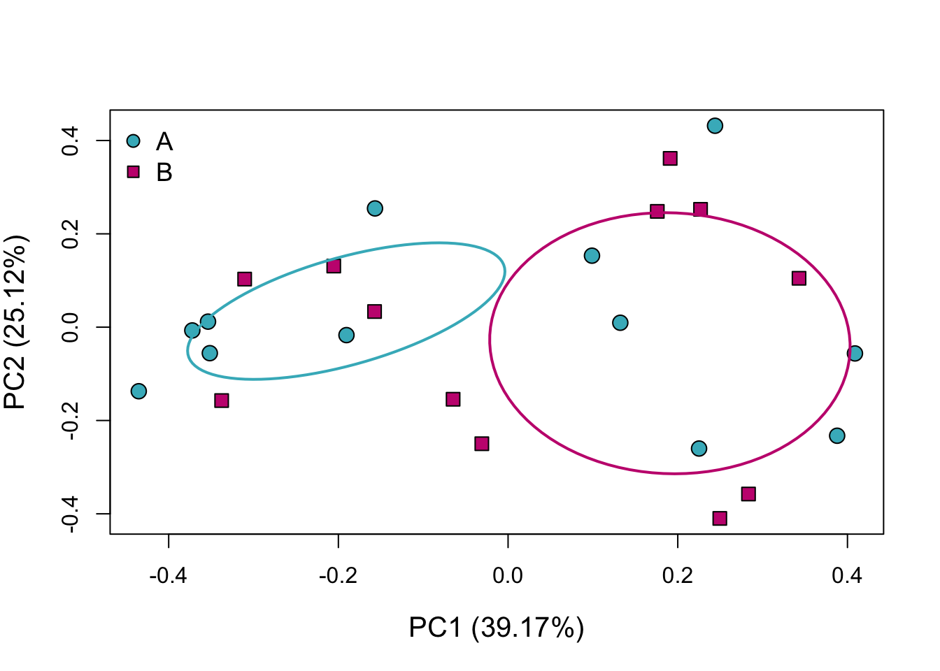
With that in hand, we can make our ordination! While you could make this step-by-step on your own, we’ll use the ordination function from the supportR package for convenience. This function automatically uses colorblind safe colors for up to 10 groups and has some useful base plot defaults (as well as including ellipses around the standard deviation of the centorid of all groups).
# Load the library
library(supportR)

# Make the ordination
supportR::ordination(mod = pcoa_points, grps = lichen_df$treatment,
1 x = "topleft", legend = c("A", "B"))- 1
- This function allows several base plot arguments to be supplied to alter non-critical plot elements (e.g., legend position, point size, etc.)

The percentages included in parentheses on either axis label are the percent of the total variation in the data explained by each axis on its own. Use this information in combination with what the graph looks like to determine how different the groups truly are.
Non-metric ordinations are typically used when you care more about the relative differences among groups rather than specific measurements between particular points. For instance, you may want to assess whether the composition of insect communities differs between two experimental treatments. In such a case, your hypothesis likely depends more on the holistic difference between the treatments rather than some quantitative difference on one of the axes.
The most common non-metric ordination type is called Nonmetric Multidimensional Scaling (NMS / NMDS). This approach prioritizes making groups that are “more different” further apart than those that are less different. However, NMS uses a dissimilarity matrix which means that the distance between any two specific points cannot be interpreted meaningfully. It is appropriate though to interpret which cloud of points is closer to/further from another in aggregate. If specific distances among points are of interest, consider a metric ordination approach.
In order to perform an NMS ordination we’ll first need to calculate a dissimilarity matrix for our response data. The vegan function metaMDS is useful for this. This function has many arguments but the most fundamental are the following:
comm= the dataframe of response variables (minus any non-numeric / grouping columns)distance= the distance/dissimilarity metric to use- Note that there is no benefit to using a metric distance because when we make the ordination it will become non-metric
k= number of axes to decompose to – typically two so the graph can be simpletry= number of attempts at minimizing “stress”- Stress is how NMS evaluates how good of a job it did at representing the true differences among groups (lower stress is better)
# Load needed libraries
library(vegan)

# Get dissimilarity matrix
dissim_mat <- vegan::metaMDS(comm = lichen_df[-1], distance = "bray", k = 2,
                             autotransform = F, expand = F, try = 50)
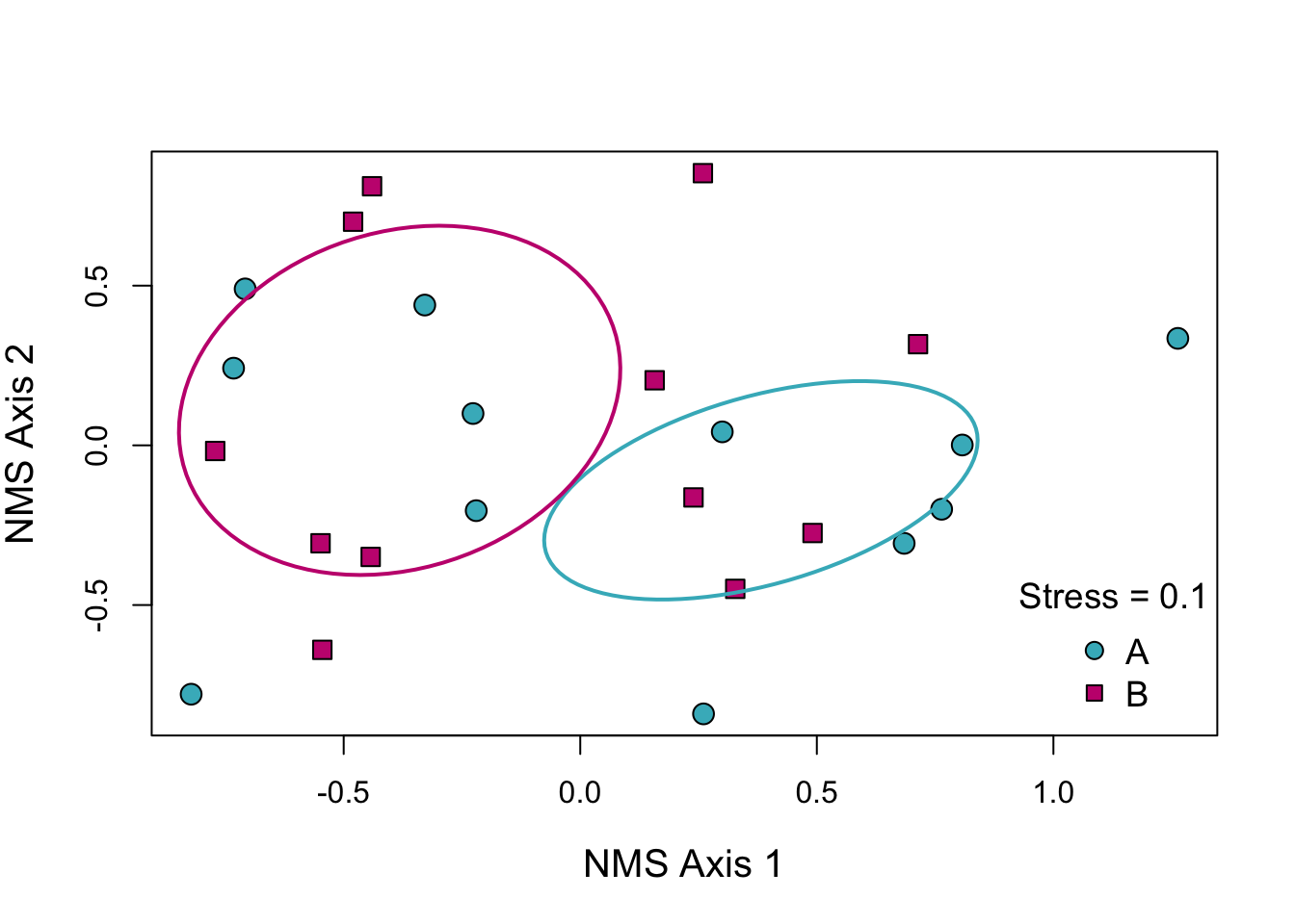
With that in hand, we can make our ordination! While you could make this step-by-step on your own, we’ll use the ordination function from the supportR package for convenience. This function automatically uses colorblind safe colors for up to 10 groups and has some useful base plot defaults (as well as including ellipses around the standard deviation of the centorid of all groups).
# Load the library
library(supportR)

# Make the ordination
supportR::ordination(mod = dissim_mat, grps = lichen_df$treatment,
1 x = "bottomright", legend = c("A", "B"))- 1
- This function allows several base plot arguments to be supplied to alter non-critical plot elements (e.g., legend position, point size, etc.)

If the stress is less than 0.15 it is generally considered a good representation of the data. We can see that the ellipses do not overlap which indicates that the community composition of our two groups does seem to differ. We’d need to do real multivariate analysis if we wanted a p-value or AIC score to support that but as a visual tool this is still useful.
Additional Resources
Papers & Documents
- Abdi, H. & Williams, L.J., Principal Coponent Analysis. WIREs Computational Statistics. 2010.
- Ramette, A., Multivariate Analyses in Microbial Ecology. FEMS Microbial Ecology. 2007.
- Jackson, D.A., Stopping Rules in Principal Components Analysis: A Comparison of Heuristical and Statistical Approaches. Ecology. 1993.
- Clarke, K.R., Non-Parametric Multivariate Analyses of Changes in Community Structure. Australian Journal of Ecology. 1993.
- Kenkel, N.C. & Oroloci, L., Applying Metric and Nonmetric Multidimensional Scaling to Ecological Studies: Some New Results. Ecology. 1986.

