Operational Synthesis

Learning Objectives

After completing this module, you will be able to:

• Summarize the advantages of creating a defined contribution workflow
• Explain how synthesis teams can use GitHub to collaborate more efficiently and reproducibly
• Identify characteristics of reproducible coding / project organization
• Explain benefits of reproducibility (to your team and beyond)
• Understand best practices for preparing and analyzing data to be used in synthesis projects

Introduction

Scientific research can be defined as “creative and systematic work undertaken in order to increase the stock of knowledge” (2015 Frascati Manual). To this basic definition of research, our definition of synthesis research adds collaborative work, and the integration and analysis of a wide range of data sources.

In Module 1 we discussed many of the collaborative considerations for synthesis research, including creating a diverse and inclusive team, asking synthesis-ready scientific questions (often broad in scope or spatial scale), and finding suitable information (or data) from a wide variety of sources to answer those questions.

Once the synthesis team moves into the operational phase of research, which includes the integration and analysis of data, there are some key activities that must happen:

1. Make a plan for technical challenges
2. Harmonize and tidy data in a reproducible way
3. Analyze data to answer your questions

Once you have analyzed your data, you can interpret the results and create products as you likely would in a non-synthesis project–though the scale and impact of your products are likely to be larger for a synthesis project than for a typical scientific effort. More on these later steps of synthesis work in Module 3.

We’ve already seen that creating a collaborative, inclusive team can set the stage for successful synthesis research. Each of the operational activities above will also benefit from this mindset, and in this module we highlight some of the most important considerations and practices for a team science approach to the nuts-and-bolts of synthesis research.

1. Make a Plan

For non-synthesis projects, it can feel intuitive to skip this step. Especially if you are working alone or with a small group of close collaborators the formal process of making and documenting your strategy can feel like a waste of time relative to ‘actually’ doing the work. However, synthesis work uses a lot of data, requires a high degree of technical collaboration, and involves a series of big judgement calls that will need to be revisited. Because of these factors, taking the time to create an actual, specific, written plan (and periodically updating that plan as priorities and questions evolve) is vital to the success of synthesis projects!

See the sub-sections below for some especially critical elements to consider as you draft your plan. Note this is not exhaustive and there will definitely be other considerations that will be reasonable for your team to add to the plan based on your project’s goals and team composition.

How Will You Get (and Stay) Organized?

Two critical elements of oragnization are (1) the folder structure on your computer of project files and (2) how you will informatively name files so their purpose is immediately apparent. Also, it is easier to start organized than it is to get organized, so implementing a system at the start of your project and sticking to it will be much easier than trying to re-organize months or years worth of work after the fact.

While there is no “one size fits all” solution to project organization, we recommend something like the following:

Key properties of this structure:

• Everything nested within a project-wide folder
• Limited use of sub-folders
• Dedicated “README” files containing high-level information about each folder
• Consistent folder/file naming conventions
  • Good names should be be both human and machine-readable (and sorted in the same way by machines and people)
  • Avoid spaces and special characters
  • Consistent use of delimeters (e.g., “-”, “_“, etc.)
• Shared file prefix (a.k.a. “slug”) connecting code files with files they create
  • Allows for easy tracing of errors because the file with issues has an explicit tie to the script that likely introduced that error
• Includes a “data log” (a.k.a. “data inventory”) for documenting data sources and critical information about each
  • E.g., dataset identifiers/DOIs, search terms used in data repository, provenance, spatiotemporal extent and granularity, etc.)

Suggested Project Structure:

synthesis_project
 |–  README.md
 |–  code
 |       |–  README.md
 |       |–  01_harmonize.R
 |        L  02_quality-control.R
 |–  data
 |       |–  README.md
 |       |–  data-log.csv
 |       |–  raw
 |        L  tidy
 |             |–  01_data-harmonized.csv
 |              L  02_data-wrangled.csv
 |–  notes
 |–  presentations
  L  publications
        |–  README.md
        |–  community-composition
         L  biogeochemistry

How Will You Collaborate?

Once you’ve decided on your organization method, you’ll need to decide as a team how you will work together. It is critical that your whole team agrees to whatever method you come up with because it will result in a lot of unnecessary work if a subset of people do not follow the plan–and thus introduce disorganization and inconsistency that someone will have to spend time fixing later.

A good rule of thumb is that you should plan for “future you.” What collaboration methods will you in 6+ months thank ‘past you’ for implementing? It may also be helpful to consider the negative side of that question: what shortcuts could you take now that ‘future you’ will be unhappy with?

A huge part of deciding how you will collaborate is deciding how you will communicate as a team. When you work asynchronously, how will you tell others that you are working on a particular code or document file? This does not have to be high tech–an email or Slack message can suffice–but if you don’t communicate about the minutiae, you risk duplicating effort or putting in conflicting work.

Where Will Code Live?

Unlike the other planning elements, we (the instructors) feel there is a single correct answer to this: your code should live in a version control system. Broadly, “version control” systems track iterative changes to files. In addition to the specific, line-by-line changes to project files, contributions of each team member are tracked, and there are straightforward systems for ‘rolling back’ files to an earlier state if needed.

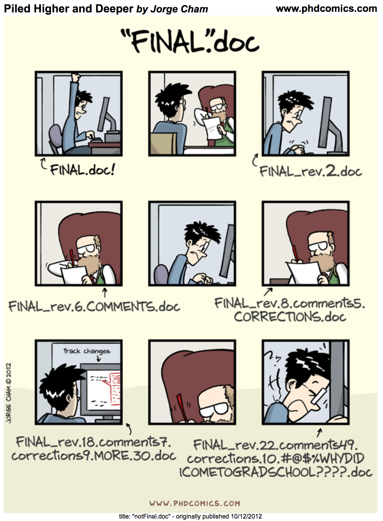
As the comic to the right shows–and as all scientists know from experience–you will have several (likely many) drafts of a given product before the finalized version. With a version control system, all the revisions in each draft are saved without needing to manually ‘re-save’ the file with a date stamp or version number in the filename. Version control systems provide a framework for preserving these changes without cluttering your computer with all of the files that precede the final version.

While there are several version control options, we recommend Git as the version control software and GitHub as the online platform for storing Git repositories in a shareable way. Note that there are viable alternatives to GitHub (e.g., GitLab, GitKraken, etc.) but (A) all of these rely on Git ‘under the hood’ and (B) in order to give an effective tutorial of version control in this course, we need to narrow our focus to just one of these website options. From here onwards, we’ll use focus on GitHub but it may be worthwhile for your team to investigate some of the GitHub alternatives as they will all offer similar functionality.

GitHub Tutorial

Given the time restrictions for this short course, we’ll only cover how you can engage with GitHub directly through its website today. However, this focus is actually a benefit to synthesis teams because learning how to engage with a Git repository via GitHub can enable collaborators who are less comfortable writing code to still fully contribute and stay abreast of the team’s progress.

There are a lot of Git/GitHub tutorials that already exist so, rather than add yet another variant to that list, we’ll instead work through part of the workshop created by the Scientific Computing team of the Long Term Ecological Research (LTER) Network Office. Note too that those materials include a detailed, step-by-step guide for working with Git/GitHub through RStudio, as well as some discussion of the project management tools that GitHub supports. As noted earlier, we won’t cover those parts of that workshop today, but they might be useful for you to revisit later.

The workshop materials we will be working through live here but for convenience we have also embedded the workshop directly into this short course’s website (see below).

2. Prepare Data

Reproducibility Practices

Making one’s work “reproducible”–particularly in code contexts–has become increasingly popular but is not always clearly defined. For the purposes of this short course, we believe that reproducible work:

• Uses scripted workflows for all interactions with data
• Contains sufficient documentation for those outside of the project team to navigate the project’s contents
• Contains detailed metadata for all data products
• Allows anyone to recreate the entire workflow from start to finish
• Leads to modular, extensible research projects. Adding data from a new site, or a new analysis, should be relatively easy in a reproducible workflow.
• External inputs are quarantined

Coding

• Use a version control system
• Load libraries/packages explicitly
• Track (and document) software versions
• Namespace functions (if not already required by your coding language)
  • E.g., dplyr::mutate(mtcars, hp_disp = hp / disp)
• Use relative file paths that are operating system-agnostic
• Balance how descriptive object names are with striving for concise names
• Use comments in the code!
• Consider custom functions
• For scripts that need to be run in order, consider adding step numbers to the file name

Synthesizing

How does reproducibility in synthesis considerations differ from individual / non-synthesis applications?

• Judgement calls need to be made / agreed to as a group
  • But “defer to the doers”
• Increased emphasis on contribution guidelines / planning being formalized
• More communication needs
• Must ensure that every team member has sufficient access to the project files
• Its best to keep track of who contributed what, so that everyone gets credit. This can be challenging in practice.

Reproducibility Questions

In groups of 3-5, discuss the following questions:

• What elements of reproducibility from our list have you used/are interested in using?
• Which feel unreasonable or confusing?
• What activities do you do in your own work to ensure reproducibility that our list is missing?

Data Preparation

The scientific questions being asked in synthesis projects are usually broad in scope, and it is therefore common to bring together many datasets from different sources for analysis. The datasets selected for analysis (source data) may have been collected by different people, in different places, using different methods, as part of different projects… or all of the above. Typically, some amount of data cleaning - filtering or removing unwanted observations - and data harmonization - putting data together in common structures, file formats, and units of measurement - is necessary before analysis can begin. This process can be easy or difficult depending on the quality of the source data, the differences between source data, and how much metadata (see callout below) is available to understand them.

Data Preparation Group Questions

• How many of you work directly with data in your day-to-day?
• What percentage of the time that you spend working on data is spent on data cleaning?
• How much on metadata creation?
• How much on data preparation?

More about Metadata

Metadata is “data about the data,” or information that describes who collected the data, what was observed or measured, when the data were collected, where the data were collected, how the observations or measurements were made, and why they were collected. Metadata provide important contextual information about the origin of the data and how they can be analyzed or used. They are most useful when attached or linked to the data being described, and data and related metadata together are commonly referred to as a dataset.

Metadata for ecological research data are well described in Michener et al (1997),¹ but there are many other kinds of metadata with different purposes.² If you are publishing a research dataset and have questions about metadata, ask a data manager for your project, or staff at the repository you are working with, for help. Either can typically provide guidance on creating metadata that will describe your data and be useful to the community (here is one example). We’ll return to the subject of metadata in Module 3.

Cleaning Data

When assembling large datasets from diverse sources, as in synthesis research, not all the source data will be useful. This may be because there are real or suspected errors, missing values, or simply because they are not needed to answer the scientific question being asked (wrong variable, different ecosystem, etc.). Data that are not useful are usually excluded from analysis or removed altogether. Data cleaning tends to be a stepwise, iterative process that follows a different path for every dataset and research project. There are some standard techniques and algorithms for cleaning and filtering data, but they are beyond the scope of this course. Below are a few guidelines to remember, and more in-depth resources for data cleaning are found at the end of this section.

1. Always preserve the raw data. Chances are you’ll want to go back and check the original source data at least once.
2. Use a scripted workflow to clean and filter the raw data, and follow the usual rules about reproducibility (comments, version control, functionalization).
3. Consider using the concept of data processing “levels,” meaning that defined sets of data flagging, removal, or transformation operations are applied consistently to the data in stepwise fashion. For example, incoming raw data would be labeled “level 0” data, and “level 1” data is reached after the first set of processing steps is applied.
4. Spread the data cleaning workload around! Data cleaning typically demands a HUGE fraction of the total time devoted to working with data,³⁴⁵ and it can be tedious work. Make sure the team shares this workload equitably.

Data Harmonization

Data harmonization is the process of bringing different datasets into a common format for analysis. The harmonized data format chosen for a synthesis project depends on the source data, analysis plans, and overall project goals. It is best to make a plan for harmonizing data BEFORE analysis begins, which means discussing this with the team in the early stages of a synthesis project. As a general rule, it is also wise to use a scripted workflow that is as reproducible as possible to accomplish the harmonization you need for your project. Following this guidance lets others understand, check, and adapt your work, and will also make it much, much easier to bring new data and analysis methods into the project.

Data harmonization is hard work that sometimes requires trial and error to arrive at a useful end product. At the end of this section are some additional data harmonization resources to help you get started. Looking at a simple example might also help.

Example: Harmonizing grassland biomass data

In the figure below, two datasets from different LTER sites have been harmonized into one file for analysis. We don’t have all the metadata here, but based on the column naming we can assume that the file on the left (Konza_harvestplots.txt, yellow) contains columns for the sampling date, a plot identifier, a treatment categorical value, and measured biomass values. The filename suggests that the data come from the Konza Prarie LTER site. The file on the right (2022_clips.csv, blue) has a column denoting the LTER site, in this case Sevilleta LTER (abbreviated as SEV), as well as similar date, plot identifier, treatment, and measured biomass columns.

There are some similarities and some differences in these two source files. A harmonized file (lter_grass_biomass_harmonized.txt) appears below.

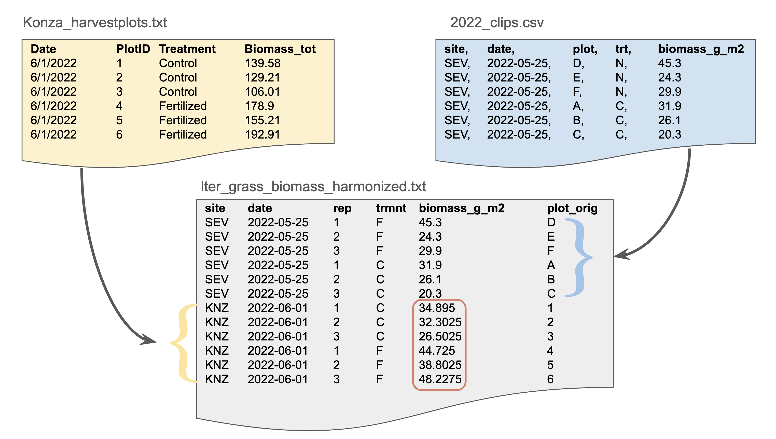
Take a minute to look at the harmonized file and consider how these data were harmonized. Then, answer the question below.

What changes were made to data structure, variable formatting, or units in these data?

Even though the source data files were similar, several important changes were made to create the harmonized file. Among them:

• The site column was preserved and contains the “SEV” and “KNZ” categorical values denoting which LTER site is observed in each row.
• The dates in the date column were converted to a standard format (YYYY-MM-DD). Incidentally, this matches the International Organization for Standardization (ISO) recommendation for date/time data, making it generally a good choice for dates.
• A new rep column was created to identify the replicate measurements at each site. This is essentially a standard version the plot identifier columns (PlotID and plot) in the original data file. Also note that the original values are preserved in the new plot_orig column.
• The treatment columns from the original data files (Treatment and trt) were standardized to one column with “C” and “F” categorical values, for control and fertilized treatments, respectively.
• The biomass values from Konza were converted to units grams per meter squared (g/m²) because the original Konza measurements were for total biomass in 2x2 meter plots. Note that this conversion is for illustration purposes only - we can’t be sure if this conversion is correct without it being spelled out in the metadata, or asking the data provider directly.

A Word about Harmonized Data Formats

Above, we have discussed several aspects of selecting a data format. There are at least three related, but not exactly equivalent, concepts to consider when formatting data. First, formats describe the way data are structured, organized, and related within a data file. For example, in a tabular data file about biomass, the measured biomass values might appear in one column, or in muiltiple columns. Second, the values of any variable can be represented in more than one format. The same date, for example, could be formatted using text as “July 2, 1974” or “1974-07-02.” Third, format may refer to the file format used to hold data on a disk or other storage medium. File formats like comma separated value text files (CSV), Excel files (.xlsx), JPEG images, are commonly used for research data, and each has particular strengths for certain kinds of data.

A few guidelines apply:

1. For formatting a tabular dataset, err towards simpler data structures, which are usually easier to clean, filter, and analyze. Long-format tables, or tidy data ⁶, is one common recommendation for this.
2. When choosing a file format, err towards open, non-proprietary file formats that more people know and have access to. Delimited text files, such as CSV files, are a good choice for tabular data.
3. Use existing community standards for formatting variables and files as long as they suit your project methods and scientific goals. Using ISO standards for date-time variables, or species identifiers from a taxonomic authority, are good examples of this practice.
4. There is no perfect data format! Harmonizing data always involves some judgement calls and tradeoffs.

When choosing a destination format for the harmonized data for a synthesis project, the audience and future uses of the data are also an important consideration. Consider how your synthesis team will analyze the data, as well as how the world outside that team will use and interact with the data once it is published. Again, there is no one answer, but below are a few examples of harmonized destination formats to consider.

Long (Tidy)

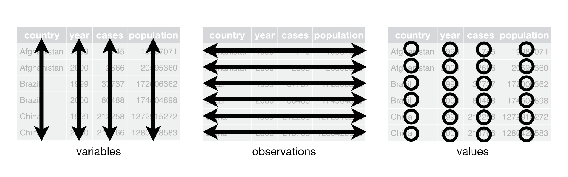
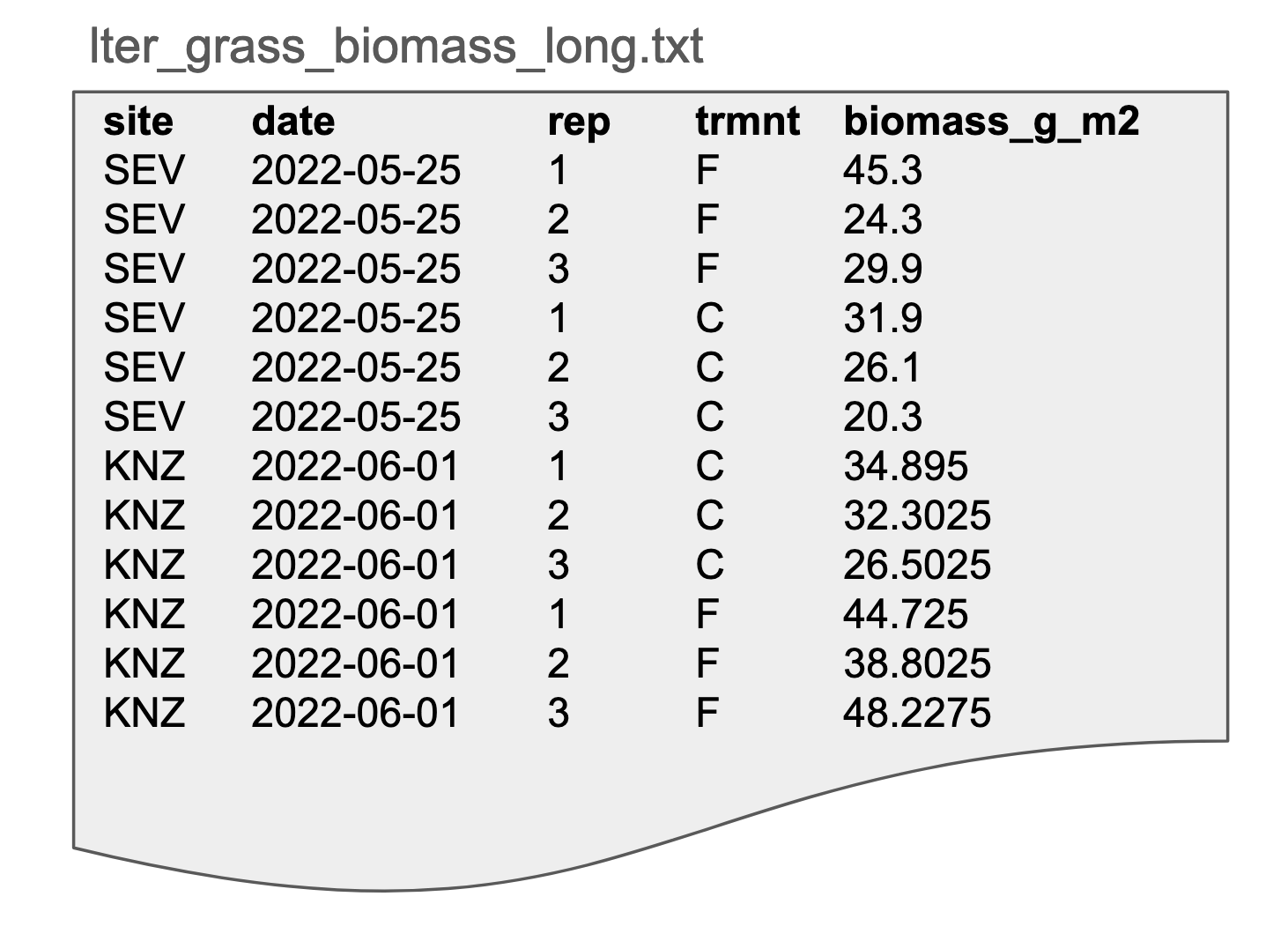
Here our grassland biomass data is in long format, often referred to as “tidy” data. Data in this format is generally easy to understand and use. There are three rules for tidy data:

1. Each column is one variable.
2. Each row is one observation.
3. Each cell contains a single value.

visual representation of the tidy data structure

Advantages: clear meaning of rows and columns; ease in filtering/cleaning/appending
Disadvantages: not as human-friendly so it can be difficult to assess the data visually
Possible file formats: Delimited text (tab delimited shown here), spreadsheets, database tables

The harmonized grassland data, in long format.

Wide (Untidy)

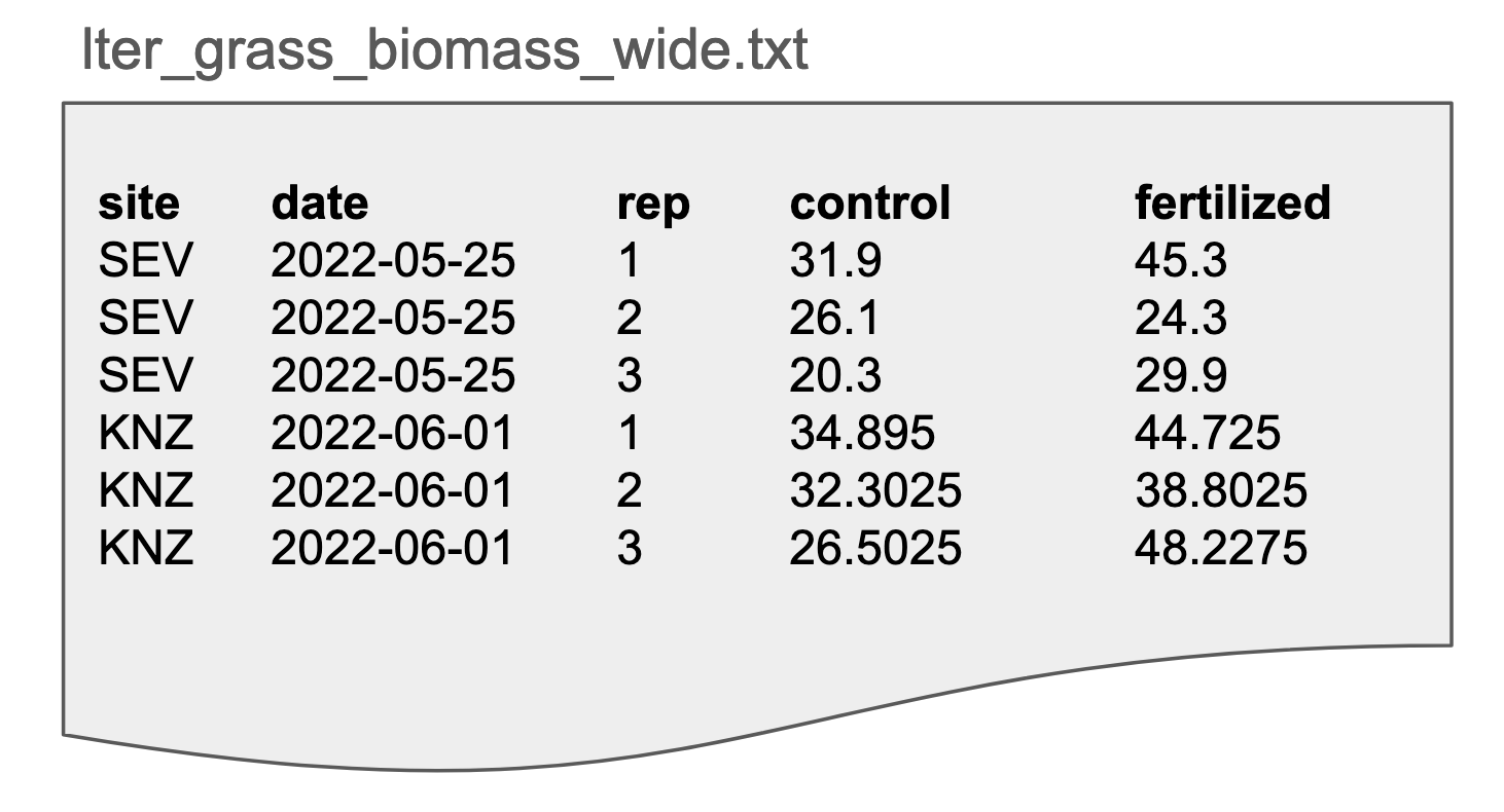
In this dataset, our grassland data has been restructured into wide format, often referred to (sometimes unfairly) as “messy” or “untidy” data. Note that the biomass variable has been split into two columns, one for control plots and one for fertilized plots.

Advantages: easier for some statistical analyses (ANOVA, for example); easier to assess the data visually
Disadvantages: may be more difficult to clean/filter/append, multiple observations per row; more likely to contain empty (NULL) cells
Possible file formats: Delimited text (tab delimited shown here), spreadsheets, database tables

The harmonized grassland data, restructured into wide format with biomass values in control and fertilized columns.

Relational Database

Below is an example of how we might structure our grassland data in a relational database. The schema consists of three tables that house information about sampling events (when, where data were collected), the plots from which the samples are collected, and the biomass values for each collection. The schema allows us to define the data types (e.g., text, integer), add constraints (e.g., values cannot be missing), and to describe relationships between tables (keys). Relational formats are normalized to reduce data redundancy and increase data integrity, which can help us to manage complex data⁷.

example grassland database schema

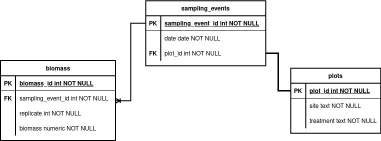
Advantages: reduced redundancy, greater integrity; community standard; powerful extensions (e.g., store and process spatial data); many different database flavors to meet specific needs
Disadvantages: significant metadata needed to describe and use; more complex to publish; learning curve
Possible file formats: Database stores, can be represented in delimited text (CSV)

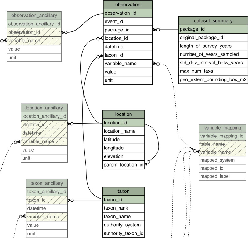
A richer example is a schematic of the related tables that comprise the ecocomDP⁸ harmonized data format for biodiversity data. Eight tables are defined, along with a set of relationships between tables (keys), and constraints on the allowable values in each table.

The ecocomDP schema. Each table has a name (top cell) and a list of columns. Shaded column names are primary keys, hashed columns have constraints, and arrows represent relations between keys/constraints in different tables.

Cloud-native

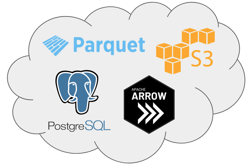
There are many possibilities to make large synthesis datasets available and useful in the cloud. These require specialized knowledge and tooling, and reliable access to cloud platforms.

Advantages: easier access to big (high volume) data, can integrate with web apps
Disadvantages: less familiar/accessible to many scientists, few best practices to follow, costs can be higher
Possible file formats: Parquet files, object storage, distributed/cloud databases

A few of the cloud-native technologies that might be useful for synthesis research products.

Other…

There are many, many other possible harmonized data formats. Here are a few possible examples:

• DarwinCore archives for biodiversity data
• Organismal trait databases
• Archives of cropped, labeled images for training machine or deep learning models
• Libraries of standardized raster imagery in Google Earth Engine

3. Analyze Data

Once the team has found sufficient source data, then harmonized, cleaned, and filtered countless datasets, and documented and described everything with quality metadata, it is finally time to analyze the data! Great! Load up R or Python and get started, and then tell us how it goes. We simply don’t have enough time to cover all the ins and outs of data analysis in a this course. However, we have put a few helpful resources below to get you started, and many of the best practices we have talked about, or will talk about, apply:

1. Document your analysis steps and comment your code, and generally try to make everything reproducible.
2. Use version control as you analyze data.
3. Give everyone a chance! Analyzing data is challenging, exciting, and a great learning opportunity. Having more eyes on the analysis process also helps catch interesting results or subtle errors.

Synthesis Group Case Studies

To make some of these concepts more tangible, let’s consider some case studies. The following tabs contain GitHub repositories for real teams that have engaged in synthesis research and chosen to preserve and maintain their scripts in GitHub. Each has different strengths and you may find that facets of each feel most appropriate for your group to adopt. There is no single “right” way of tackling this but hopefully parts of these exemplars inspire you.

Example 1

LTER SPARC Group: Soil Phosphorus Control of Carbon and Nitrogen

Stored their code here: lter / lter-sparc-soil-p

Highlights

• Straightforward & transparent numbering of workflow scripts
  • File names also reasonably informative even without numbering
• Simple README in each folder written in human-readable language
• Custom .gitignore safety net
  • Controls which files are “ignored” by Git (prevents accidentally sharing data/private information)

Example 2

LTER Full Synthesis Working Group: The Flux Gradient Project

Stored their code here: lter / lterwg-flux-gradient

Highlights

• Extremely consistent file naming conventions
• Strong use of sub-folders for within-project organization
• Top-level README includes robust description of naming convention, folder structure, and order of scripts in workflow
• Active contribution to code base by nearly all group members
  • Facilitated by strong internal documentation and consenus-building prior to choosing this structure

Example 3

LTER Full Synthesis Working Group: From Poles to Tropics: A Multi-Biome Synthesis Investigating the Controls on River Si Exports

Stored their code here: lter / lterwg-silica-spatial

Highlights

• Files performing similar functions share a prefix in their file name
• Use of GitHub “Release” feature to get a persistent DOI for their codebase
• Separate repositories for each manuscript
• Nice use of README as pseudo-bookmarks for later reference to other repositories

For more information about LTER synthesis working groups and how you can get involved in one, click here.

Additional Resources

Data Preparation

Data cleaning and filtering resources

• Data cleaning is complicated and varied, and entire books have been written on the subject.⁹¹⁰ For some general considerations on cleaning data, see EDI’s “Cleaning Data and Quality Control” resource
• OpenRefine is an open-source, cross-platform tool for iterative, scripted data cleaning.
• In the R language, the tidyverse libraries (particularly tidyr and dplyr) are often used for data cleaning, as are additional libraries like janitor.
• In Python, pandas and numpy libraries provide useful data cleaning features. There are also some stand-alone cleaning tools like pyjanitor (started as a re-implementation of the R version) and cleanlab (geared towards machine learning applications).
• Both the R and Python data science ecosystems have excellent documentation resources that thoroughly cover data cleaning. For R, consider starting with Hadley Wickham’s R for Data Science book chapter on data tidying,¹¹ and for python check Wes McKinney’s Python for Data Analysis book chapter on data cleaning and preparation.¹²

Data harmonization resources

• For R and Python users, there are, again, excellent documentation resources that thoroughly cover data harmonization techniques like data filtering, reformatting, joins, and standardization. In Hadley Wickham’s R for Data Science book, the chapters on data transforms and data tidying are a good place to start. In Wes McKinney’s Python for Data Analysis book, the chapter on data wrangling is helpful.
• A nice article in “The Analysis Factor” describes wide vs long data formats and when to choose which (TLDR, it depends on your statistical analysis plan).

Data Analysis

• Harrer, M. et al. Doing Meta-Analysis with R: A Hands-On Guide. 2023. GitHub
• Once again, for R and Python users, the same two books mentioned above provide excellent beginning guidance on data analysis techniques (exploratory analysis, summary stats, visualization, model fitting, etc). In Wickham’s R for Data Science book, the chapter on exploratory data analysis will help. In McKinney’s Python for Data Analysis book, try the chapters on plotting and visualization and the introduction to modeling.

Courses, Workshops, and Tutorials

• Synthesis Skills for Early Career Researchers (SSECR) course. 2024. LTER Network Office
• Reproducible Approaches to Arctic Research Using R workshop. 2024. Arctic Data Center & NCEAS Learning Hub
• Collaborative Coding with GitHub workshop. 2024. NCEAS Scientific Computing team
• Coding in the Tidyverse workshop. 2023. NCEAS Scientific Computing team
• Shiny Apps for Sharing Science workshop. 2022. Lyon, N.J. et al.
• Ten Commandments for Good Data Management. 2016. McGill, B.

Literature

• Todd-Brown, K.E.O., et al. Reviews and Syntheses: The Promise of Big Diverse Soil Data, Moving Current Practices Towards Future Potential. 2022. Biogeosciences
• Borer, E.T. et al. Some Simple Guidelines for Effective Data Management. 2009. Ecological Society of America Bulletin

Other

• Better commit messages with Conventional Commits

Footnotes

1. Michener, W.K., Brunt, J.W., Helly, J.J., Kirchner, T.B. and Stafford, S.G. (1997), NONGEOSPATIAL METADATA FOR THE ECOLOGICAL SCIENCES. Ecological Applications, 7: 330-342. https://doi.org/10.1890/1051-0761(1997)007[0330:NMFTES]2.0.CO;2

2. Mayernik, M.S. and Acker, A. (2018), Tracing the traces: The critical role of metadata within networked communications. Journal of the Association for Information Science and Technology, 69: 177-180. https://doi.org/10.1002/asi.23927

3. Wickham, H. (2014). Tidy Data. Journal of Statistical Software, 59(10), 1–23. https://doi.org/10.18637/jss.v059.i10

4. New York Times, 2014

5. Anaconda State of Data Science Report, 2022

6. Wickham, H. (2014). Tidy Data. Journal of Statistical Software, 59(10), 1–23. https://doi.org/10.18637/jss.v059.i10

7. Zimmerman, N. 2016. Hand-crafted relational databases for fun and science

8. O’Brien, Margaret, et al. “ecocomDP: a flexible data design pattern for ecological community survey data.” Ecological Informatics 64 (2021): 101374. https://doi.org/10.1016/j.ecoinf.2021.101374

9. Osborne, Jason W. Best practices in data cleaning: A complete guide to everything you need to do before and after collecting your data. Sage publications, 2012.

10. Van der Loo, Mark, and Edwin De Jonge. Statistical data cleaning with applications in R. John Wiley & Sons, 2018. https://doi.org/10.1002/9781118897126

11. Wickham, Hadley, Mine Çetinkaya-Rundel, and Garrett Grolemund. R for data science. ” O’Reilly Media, Inc.”, 2023. https://r4ds.hadley.nz/

12. McKinney, Wes. Python for data analysis. ” O’Reilly Media, Inc.”, 2022. https://wesmckinney.com/book